What is Time Series?#
by Professor Throckmorton
for Time Series Econometrics
W&M ECON 408/PUBP 616
Slides
Definition#
A time series is a sequence of data points collected over time.
These data points are ordered by time, and the sequence of the data cannot be interchanged.
Time series analysis focuses on transforming, visualizing, and modeling this type of data.
When modeling a time series, its value at any time is random, i.e., the realization of a random variable.
Thus, a time series is a discrete stochastic process.
Plots#
A time series plot (or time plot) is a graph that visualizes the evolution of a time series.
Time, \(t\), is on the horizontal axis.
Observed values are on the vertical axis.
Time series plots are crucial for analysis, revealing patterns such as trend and seasonality.
The first step always is to plot the recorded data and do a visual examination, i.e., “eyeball econometrics.”
For economic time series data, usually we have observations at regular intervals, or frequencies, e.g., daily, monthly, quarterly, or annual.
Examples#
Daily:
Monthly:
Quarterly: U.S. Gross Domestic Product (GDP)
Annual: U.S. Capital Stock
# Libraries
from fredapi import Fred
import pandas as pd
# Read Data
fred_api_key = pd.read_csv('fred_api_key.txt', header=None)
fred = Fred(api_key=fred_api_key.iloc[0,0])
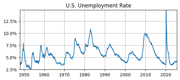
data = fred.get_series('UNRATE').to_frame(name='UR')
print(data.head(2))
print(data.tail(2))
             UR
1948-01-01  3.4
1948-02-01  3.8
             UR
2025-07-01  4.2
2025-08-01  4.3
# Plotting
import matplotlib.pyplot as plt
# Plot
fig, ax = plt.subplots(figsize=(6.5,2.5));
ax.plot(data.UR);
ax.set_title('U.S. Unemployment Rate');
ax.yaxis.set_major_formatter('{x:,.1f}%')
ax.grid(); ax.autoscale(tight=True)
Objectives#
Time series plots are useful for identifying
trends, i.e., long-term systematic patterns.
seasons, i.e., common patterns across years.
cycles, i.e, patterns related to economic recessions and expansions.
structural changes to trend, seasonal, or cyclical patterns.
outliers (anomalies).
Descriptive statistics are used to summarize the properties of time series, e.g., Mean/Expected Value, Variance/Std. Deviation, Autocorrelation, Skewness, Kurtosis, percentiles, and min/max are all useful descriptive statistics.
# Import libraries
#   Scientific computing, statistical functions
import scipy.stats as stats

# Mean
print(f'Most recent UR = {data.UR.iloc[-1]:.1f}%')
print(f'E(UR) = {stats.tmean(data.UR):.1f}%')
print(f'Std(UR) = {stats.tstd(data.UR):.1f}%')
print(f'Skew(UR) = {stats.skew(data.UR):.1f}')
print(f'Kurt(UR) = {stats.kurtosis(data.UR):.1f}')
print(f'min(UR) = {data.UR.min():.1f}%')
print(f'max(UR) = {data.UR.max():.1f}%')
Most recent UR = 4.3%
E(UR) = 5.7%
Std(UR) = 1.7%
Skew(UR) = 0.9
Kurt(UR) = 1.1
min(UR) = 2.5%
max(UR) = 14.8%
# Plot histogram
fig, ax = plt.subplots(figsize=(6.5,2.5));
ax.hist(data.UR,edgecolor='black',density='true')
ax.set_xlabel('U.S. Unemployment Rate');
ax.set_ylabel('probability')
ax.xaxis.set_major_formatter('{x:,.1f}%')
ax.grid(); ax.autoscale(tight=True)
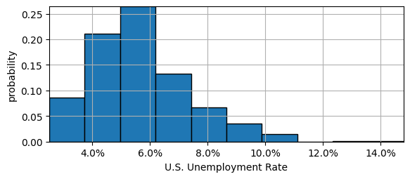
Most recent UR is \(4.1\%\), or \(1.6pp\) below historical mean of \(5.7\%\)
Std. Dev. is \(1.7\%\). If UR was normally distributed, then \(\pm 2 SD\), or interval from \(0.7\%\) to \(9.1\%\), would contain \(95\%\).
But minimum UR is \(2.5\%\) and maximum is \(14.8\%\), which indicates UR is most likely skewed.
\(Skew(UR) = 0.9\) and we see that histogram has long right tail.
Key Concepts#
White Noise is a special type of time series, where the values are random and uncorrelated across time.
Stationarity, e.g., does the data have a trend, seasonality, or is the covariance changing over time? If no to all, then it is stationary.
If the data is non-stationary, then the underlying probabilistic structure of the series is changing over time, and there is no way to relate the future to the past.
A Random Walk is a key model for the log price of a financial asset.
Autocorrelation is a measure of how values in a time series are correlated with previous values.