Review 1B Key#
by Professor Throckmorton
for Time Series Econometrics
W&M ECON 408/PUBP 616
Slides
1)#
Read U.S. Industrial Production: Total Index (
IPB50001N) from FRED.Resample/reindex the data to a quarterly frequency using the value for the last month of each quarter.
Print the original data and compare it to the resampled/reindexed data to verify it is correct.
# Libraries
from fredapi import Fred
import pandas as pd
# Read data
fred_api_key = pd.read_csv('fred_api_key.txt', header=None)
fred = Fred(api_key=fred_api_key.iloc[0,0])
data = fred.get_series('IPB50001N').to_frame(name='IP')
print(data.tail(3))
# Resample/reindex to quarterly frequency
data = data.resample('QE').last()
# Print data
print(f'number of rows/quarters = {len(data)}')
print(data.tail(3))
                  IP
2025-06-01  105.4026
2025-07-01  104.3398
2025-08-01  106.0004
number of rows/quarters = 427
                  IP
2025-03-31  104.1248
2025-06-30  105.4026
2025-09-30  106.0004
2)#
Why is this data not stationary?
Use appropriate transformations to remove the non-stationarity and plot the series.
Correctly and completely label the plot.
# Plotting
import matplotlib.pyplot as plt
# Plot
fig, ax = plt.subplots(figsize=(6.5,2));
ax.plot(data.IP);
ax.set_title('Industrial Production (Index, Quarterly)');
ax.grid(); ax.autoscale(tight=True)
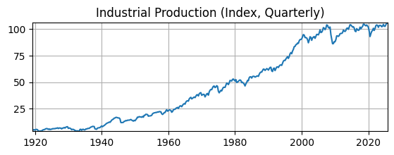
This data is non-stationary because it is seasonal over the year and it has an exponential time trend.
# Scientific computing
import numpy as np
# Transform data
#    Take log
data['logIP'] = np.log(data.IP)
#    Take difference
data['dlogIP'] = 100*(data.logIP.diff(4))
# Plot
fig, ax = plt.subplots(figsize=(6.5,2.5));
ax.plot(data.dlogIP);
ax.set_title('Industrial Production (YoY % Change, Quarterly)');
ax.yaxis.set_major_formatter('{x:.0f}%')
ax.grid(); ax.autoscale(tight=True)
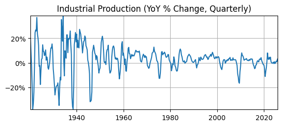
Time varying volatility indicates this is non-stationary data.
3)#
Plot the autocorrelation function of the transformed data.
Is it stationary? Why or why not?
#   Auto-correlation function
from statsmodels.graphics.tsaplots import plot_acf as acf
# Plot Autocorrelation Function
fig, ax = plt.subplots(figsize=(6.5,2))
acf(data.dlogIP.dropna(),ax)
ax.grid(); ax.autoscale(tight=True)
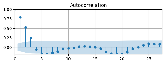
ACF is signifcant at long lags, doesn’t clearly taper to zero
might be non-stationary
First 3 lags are remarkable
4)#
Conduct a unit root test of the transformed data.
Is it stationary? Why or why not?
# ADF Test
from statsmodels.tsa.stattools import adfuller
# Function to organize ADF test results
def adf_test(data):
    keys = ['Test Statistic','p-value','# of Lags','# of Obs']
    values = adfuller(data)
    test = pd.DataFrame.from_dict(dict(zip(keys,values[0:4])),
                                  orient='index',columns=[data.name])
    return test
adf_test(data.dlogIP.dropna())
| dlogIP | |
|---|---|
| Test Statistic | -5.814992e+00 |
| p-value | 4.313232e-07 |
| # of Lags | 1.500000e+01 |
| # of Obs | 4.070000e+02 |
Null hypothesis: data has unit root
p-value near zero, so reject the null
Unit root test says data is probably stationary
5)#
If you were to pick a parsimonious AR model (i.e., the number of lags is less than 5) to fit the transformed data, what lag would you pick? Why?
# Partial auto-correlation function
from statsmodels.graphics.tsaplots import plot_pacf as pacf
# Plot Autocorrelation Function
fig, ax = plt.subplots(figsize=(6.5,1.5))
pacf(data.dlogIP.dropna(),ax)
ax.grid(); ax.autoscale(tight=True);
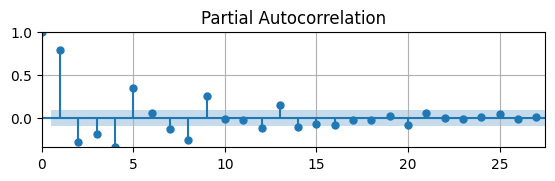
PACF is signficantly different from zero for first 5 lags
Stops being signficant for lag 6
6)#
Given your last answer, estimate an AR model given the transformed quarterly data.
Interpret the results.
# ARIMA model
from statsmodels.tsa.arima.model import ARIMA
# Define model
mod = ARIMA(data.dlogIP,order=(5,0,0))
# Estimate model
res = mod.fit()
summary = res.summary()
# Print summary tables
tab0 = summary.tables[0].as_html()
tab1 = summary.tables[1].as_html()
tab2 = summary.tables[2].as_html()
#print(tab0); print(tab1); print(tab2)
| Dep. Variable: | dlogIP | No. Observations: | 425 |
|---|---|---|---|
| Model: | ARIMA(5, 0, 0) | Log Likelihood | -1298.814 |
| coef | std err | z | P>|z| | [0.025 | 0.975] | |
|---|---|---|---|---|---|---|
| const | 2.9265 | 0.975 | 3.002 | 0.003 | 1.016 | 4.837 |
| ar.L1 | 1.0243 | 0.031 | 32.647 | 0.000 | 0.963 | 1.086 |
| ar.L2 | -0.1735 | 0.042 | -4.163 | 0.000 | -0.255 | -0.092 |
| ar.L3 | 0.1902 | 0.035 | 5.505 | 0.000 | 0.123 | 0.258 |
| ar.L4 | -0.6642 | 0.029 | -22.871 | 0.000 | -0.721 | -0.607 |
| ar.L5 | 0.3486 | 0.025 | 13.773 | 0.000 | 0.299 | 0.398 |
| sigma2 | 27.8385 | 0.912 | 30.511 | 0.000 | 26.050 | 29.627 |
| Heteroskedasticity (H): | 0.05 | Skew: | 0.34 |
|---|---|---|---|
| Prob(H) (two-sided): | 0.00 | Kurtosis: | 13.72 |
All the AR coefficients are significantly different than zero
Residuals have a lot of kurtosis, so maybe AR model isn’t the best choice