VECM#
by Professor Throckmorton
for Time Series Econometrics
W&M ECON 408/PUBP 616
Slides
Summary#
Vector Error Correction Model (VECM) is specifically used for analyzing cointegrated time series that are first-order integrated, I(\(1\)).
VECM is builds on the concept of cointegration, i.e., each time series might be I(\(1\)), and certain linear combinations of them are stationary, I(\(0\)).
VECM is derived from a reduced-form VAR in levels when the data is cointegrated
VECM includes an error correction term that reflects the deviation from the lagged long-run average or “equilibrium”
VECM#
Suppose \(\mathbf{y}_t\) is a VAR(\(p\)) with I(\(1\)), possibly cointegrated, variables in levels, then
\[\begin{gather*} \Delta \mathbf{y}_t = \boldsymbol{\Pi} \mathbf{y}_{t-1} + \sum_{h=1}^{p-1} \boldsymbol{\Gamma}_h \Delta \mathbf{y}_{t-h} + \boldsymbol{\upsilon}_t \end{gather*}\]\(\Delta \mathbf{y}_t\) is the first difference of a vector of \(n\) non-stationary, I(\(1\)), variables, making them stationary. \(\sum_{h=1}^{p-1} \boldsymbol{\Gamma}_h \Delta \mathbf{y}_{t-h}\) captures the short-run dynamics of the system, and \(\boldsymbol{\upsilon}_t\) is a vector of white noise errors.
\(\boldsymbol{\Pi} \mathbf{y}_{t-1}\) is the error correction term, i.e., the long-run equilibrium relationship between variables in levels, where \(\boldsymbol{\Pi}\) is the cointegration structure.
If \(\boldsymbol{\Pi} = \boldsymbol{0}\), there is no cointegration and no need for VECM.
If \(\boldsymbol{\Pi}\) has reduced rank, \(r < n\), then \(\boldsymbol{\Pi} = \boldsymbol{\alpha} \boldsymbol{\beta}'\), where:
\(\boldsymbol{\beta}_{n \times r}\) is a matrix of cointegrating vectors.
\(\boldsymbol{\alpha}_{n \times r}\) is a matrix of adjustment coefficients, determining how each variable returns to its long-run equilibrium.
If \(\boldsymbol{\Pi}\) is full rank, \(r = n\), then \(\mathbf{y}_t\) is already stationary and no need for VECM.
Rank of a matrix#
A square matrix \(\mathbf{A}_{n \times n}\) is full rank if its rank is \(n\). It’s not full rank, or has reduced rank, if its rank \(<n\).
The following conditions are all equivalent — if any one is true, the matrix is full rank (warning: this is not a complete list)
Linearly independent columns: No column can be written as a linear combination of the others.
Linearly independent rows: No row is a linear combination of other rows.
Non-zero determinant: \(\det(\mathbf{A}) \ne 0\) or \(|\mathbf{A}| \ne 0\)
Invertibility: there exists \(\mathbf{A}^{-1}\) such that \(\mathbf{A} \mathbf{A}^{-1} = I_n\)
Examples#
Consider the following square matrix
\[\begin{gather*} \mathbf{A} = \begin{bmatrix} 2 & 4 \\ 1 & 2 \end{bmatrix} \end{gather*}\]Column 2 is \(2\times\) column 1 \(\rightarrow\) \(\mathbf{A}\) is not full rank
Row 1 is \(2\times\) row 2 \(\rightarrow\) \(\mathbf{A}\) is not full rank
Consider the following square matrix
\[\begin{gather*} \mathbf{A} = \begin{bmatrix} 3 & 5 \\ 2 & 4 \end{bmatrix} \end{gather*}\]We can’t multiply one row or column by a constant to get the other.
The determinant of a \(2 \times 2\) matrix is \(|\mathbf{A}| = ad - bc\)
Plug in the values \(|\mathbf{A}| = (3)(4) - (5)(2) = 12 - 10 = 2\)
Since \(|\mathbf{A}| \neq 0\), the matrix is full rank.
# Scientific computing
import numpy as np
# Matrix
A = np.array([
    [1, 2],
    [2, 4]
])
# Rank
rank = np.linalg.matrix_rank(A)
# Determinant
det = np.linalg.det(A)
# Display
print(f'det = {det:.4f}')
print(rank)
det = 0.0000
1
# Matrix
A = np.array([
    [3, 5],
    [2, 4]
])
# Rank
rank = np.linalg.matrix_rank(A)
# Determinant
det = np.linalg.det(A)
# Display
print(f'det = {det:.4f}')
print(rank)
det = 2.0000
2
For a \(3 \times 3\) square matrix
\[\begin{gather*} \mathbf{A} = \begin{bmatrix} a & b & c \\ d & e & f \\ g & h & i \end{bmatrix} \end{gather*}\]The determinant formula is \(a(ei - fh) - b(di - fg) + c(dh - eg)\).
That is the sum of the three determinants for \(2 \times 2\) matrices.
Cointegration#
If some linear combination of non-stationary I(\(1\)) time series is stationary, then the variables are cointegrated, i.e., they share a stable long-run linear relationship despite short-run fluctuations.
Suppose we want to test for how many cointegrating relationships, \(r\), exist among \(n\), I(\(1\)), time series.
For example, if \(r = 0\), then there are no cointegrating relationships, and if \(r=n-1\) then all variables are cointegrated with eachother.
To justify estimating a VECM, there should be at least one cointegrating relationship between the variables, otherwise just esimate a VAR after first differencing.
Johansen Cointegration Test#
First, use the ADF (unit root) test to confirm that all time series are I(\(1\)).
The Johansen Cointegration Test has nested hypotheses
Suppose there are \(r_0 = 0\) cointegrating relationships
Null Hypothesis: \(H_0: r \leq r_0\) (i.e., the number of cointegrating relationships \(\leq r_0\))
Alternative Hypothesis: \(H_A: r > r_0\)
For each null hypothesis \(H_0: r \leq r_0\), if the test statistic \(>\) critical value \(\Rightarrow\) reject \(H_0\).
Then update \(r_0 = 1,2,3,\ldots\) until test fails to reject
In practice, use
coint_johansen()function fromstatsmodels.tsa.vector_ar.vecm.Choose lag length (\(p-1\)) for the VAR in differences.
Decide on deterministic components (constant/time trend) in the test.
Proceed to estimate a VECM if cointegration is found.
Example#
The U.S. macroeconomy has gone through many important generational changes that might affect the cointegrating relationships between aggregate time series variables
E.g, The Great Depression, Post-War Period, Great Inflation of the late 1960s to early 1980s, The Great Moderation, The Great Recession (and the slow recovery), Post COVID
Let’s test whether consumption and income are cointegrated for the 25 years prior to the Great Moderation (1960-1984)
Measure them with log real PCE and log real GDP
Read Data#
# Libraries
from fredapi import Fred
import pandas as pd
# Setup acccess to FRED
fred_api_key = pd.read_csv('fred_api_key.txt', header=None).iloc[0,0]
fred = Fred(api_key=fred_api_key)
# Series to get
series = ['GDP','PCE','GDPDEF']
rename = ['gdp','cons','price']
# Get and append data to list
dl = []
for idx, string in enumerate(series):
    var = fred.get_series(string).to_frame(name=rename[idx])
    dl.append(var)
    print(var.head(2)); print(var.tail(2))
            gdp
1946-01-01  NaN
1946-04-01  NaN
                  gdp
2025-01-01  30042.113
2025-04-01  30485.729
             cons
1959-01-01  306.1
1959-02-01  309.6
               cons
2025-07-01  20982.7
2025-08-01  21111.9
             price
1947-01-01  11.141
1947-04-01  11.299
              price
2025-01-01  127.577
2025-04-01  128.248
Create Dataframe#
# Concatenate data to create data frame (time-series table)
raw = pd.concat(dl, axis=1).sort_index()
# Resample/reindex to quarterly frequency
raw = raw.resample('QE').last()
# Display dataframe
display(raw.head(2))
display(raw.tail(2))
| gdp | cons | price | |
|---|---|---|---|
| 1946-03-31 | NaN | NaN | NaN |
| 1946-06-30 | NaN | NaN | NaN |
| gdp | cons | price | |
|---|---|---|---|
| 2025-06-30 | 30485.729 | 20868.4 | 128.248 |
| 2025-09-30 | NaN | 21111.9 | NaN |
Transform Data#
data = pd.DataFrame()
# log real GDP
data['logGDP'] = 100*(np.log(raw['gdp']/raw['price']))
data['dlogGDP'] = data['logGDP'].diff(1)
# log real Consumption
data['logCons'] = 100*(np.log(raw['cons']/raw['price']))
data['dlogCons'] = data['logCons'].diff(1)
# Select sample
sample = data['01-01-1960':'12-31-1984']
display(sample.head(2))
display(sample.tail(2))
| logGDP | dlogGDP | logCons | dlogCons | |
|---|---|---|---|---|
| 1960-03-31 | 356.027682 | 2.226717 | 306.351449 | 1.839417 |
| 1960-06-30 | 355.485842 | -0.541840 | 306.068692 | -0.282757 |
| logGDP | dlogGDP | logCons | dlogCons | |
|---|---|---|---|---|
| 1984-09-30 | 441.310256 | 0.959766 | 393.568460 | 0.634225 |
| 1984-12-31 | 442.127526 | 0.817270 | 394.731279 | 1.162819 |
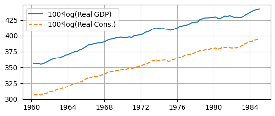
Plot Sample#
# Data in levels
sample_lev = sample[['logGDP','logCons']]
# Plot data
import matplotlib.pyplot as plt
fig, ax = plt.subplots(figsize=(6.5,2.5))
ax.plot(sample_lev['logGDP'],
        label='100*log(Real GDP)', linestyle='-')
ax.plot(sample_lev['logCons'],
        label='100*log(Real Cons.)', linestyle='--')
ax.grid(); ax.legend(loc='upper left');
ADF Unit Root Test#
from statsmodels.tsa.stattools import adfuller
# Function to organize ADF test results
def adf_test(data,const_trend):
    keys = ['Test Statistic','p-value','# of Lags','# of Obs']
    values = adfuller(data,regression=const_trend)
    test = pd.DataFrame.from_dict(dict(zip(keys,values[0:4])),
                                  orient='index',columns=[data.name])
    return test
dl = []
for column in sample.columns:
    test = adf_test(sample[column],const_trend='c')
    dl.append(test)
results = pd.concat(dl, axis=1)
display(results)
| logGDP | dlogGDP | logCons | dlogCons | |
|---|---|---|---|---|
| Test Statistic | -1.341693 | -4.949552 | -1.158324 | -5.421674 |
| p-value | 0.609889 | 0.000028 | 0.691262 | 0.000003 |
| # of Lags | 2.000000 | 1.000000 | 2.000000 | 1.000000 |
| # of Obs | 97.000000 | 98.000000 | 97.000000 | 98.000000 |
Note: the argument
const_trendsets whether the test accounts for a constant,'c', and time trend,'ct'.Fail to reject null for both time series in levels
Reject the null for both first-differenced time series
Since they are both \(I(1)\), proceed to Johansen Cointegration Test
Trends#
Stochastic trend, i.e., \(y_t = \mu + y_{t-1} + \varepsilon_t\)
Can drift without bound — non-stationary
Deterministic trend, i.e., \(y_t = \mu + \delta t + \varepsilon_t\)
Deviations from the time trend are mean-reverting
Both deterministic and stochastic trends, i.e., \(y_t = \mu + \delta t + y_{t-1} + \varepsilon_t\)
First differencing will remove either trend.
# Test data for deterministic time trend
dl = []
for column in sample_lev.columns:
    test = adf_test(sample_lev[column],'ct')
    dl.append(test)
results = pd.concat(dl, axis=1)
display(results)
| logGDP | logCons | |
|---|---|---|
| Test Statistic | -2.482304 | -2.202394 |
| p-value | 0.336865 | 0.488503 |
| # of Lags | 2.000000 | 2.000000 |
| # of Obs | 97.000000 | 97.000000 |
In
adfuller, settingregression = 'ct'allows for both a constant and linear time trend.Fail to reject the null that the data (after removing linear trend) has a unit root, i.e., removing the linear trend did not make the data stationary.
The data is probably stationary around a stochastic trend.
Regardless, first differencing the data for the VECM will remove these trends, so we don’t need to account for them later.
Cointegration Test#
# Johansen Cointegration Test
from statsmodels.tsa.vector_ar.vecm import coint_johansen
test = coint_johansen(sample_lev, det_order=-1, k_ar_diff=1)
test_stats = test.lr1; crit_vals = test.cvt[:, 1]
# Print results
for r_0, (test_stat, crit_val) in enumerate(zip(test_stats, crit_vals)):
    print(f'H_0: r <= {r_0}')
    print(f'  Test Stat. = {test_stat:.2f}, 5% Crit. Value = {crit_val:.2f}')
    if test_stat > crit_val:
        print('  => Reject null hypothesis.')
    else:
        print('  => Fail to reject null hypothesis.')
H_0: r <= 0
  Test Stat. = 34.30, 5% Crit. Value = 12.32
  => Reject null hypothesis.
H_0: r <= 1
  Test Stat. = 0.03, 5% Crit. Value = 4.13
  => Fail to reject null hypothesis.
There is evidence that GDP and consumption are cointegrated.
det_order = -1omits a common constant or linear time trend from the cointegrating relationship.k_ar_diff = 1means we are using a VECM with 1 lag of differences.
Estimation#
There is evidence that both GDP and consumption are I(\(1\)) and they are cointegrated.
If the data wasn’t cointegrated, they should be first differenced and estimate a VAR instead.
Proceed with estimating a bivariate VECM
\[\begin{align*} \Delta \tilde{y}_{t} &= \mu_1 + \alpha_1 (\beta_1 \tilde{y}_{t-1} + \beta_2 \tilde{c}_{t-1}) + \Gamma_{11} \Delta \tilde{y}_{t-1} + \Gamma_{12} \Delta \tilde{c}_{t-1} + \cdots + \varepsilon_{1,t} \\ \Delta \tilde{c}_{t} &= \mu_2 + \alpha_2 (\beta_1 \tilde{y}_{t-1} + \beta_2 \tilde{c}_{t-1}) + \Gamma_{21} \Delta \tilde{y}_{t-1} + \Gamma_{22} \Delta \tilde{c}_{t-1} + \cdots +\varepsilon_{2,t} \end{align*}\]where \(\tilde{y} =\) log real GDP and \(\tilde{c} =\) log real PCE and \(\beta_1 \tilde{y}_{t-1} + \beta_2 \tilde{c}_{t-1}\) is their cointegrating relationship.
Model Selection#
# Select number of lags in VECM
from statsmodels.tsa.vector_ar.vecm import select_order
lag_order_results = select_order(
    sample_lev, maxlags=8, deterministic='co')
print(f'Selected lag order (AIC) = {lag_order_results.aic}')
Selected lag order (AIC) = 1
In select_order:
deterministicsets which deterministic terms appear in the VECM, e.g.,deterministic = 'co'puts a constant outside the error correction to estimate the intercept since \(\Delta \tilde{y}_{t}\) and \(\Delta \tilde{c}_{t}\) have non-zero meansSelection criterion for lag order includes AIC and BIC (among others)
# Determine number of cointegrating relationships
from statsmodels.tsa.vector_ar.vecm import select_coint_rank
coint_rank_results = select_coint_rank(
    sample_lev, method='trace', det_order=-1, k_ar_diff=lag_order_results.aic)
print(f'Cointegration rank = {coint_rank_results.rank}')
Cointegration rank = 1
In select_coint_rank:
method='trace'uses the Johansen Cointegration Testdet_order=-1means there are not any deterministic terms in the cointegrating relationship(s), which is the same assumption as above when we usedcoint_johansendirectly (above).k_ar_diffis set to result of the AIC selection criterion.
Results#
from statsmodels.tsa.vector_ar.vecm import VECM
# Estimate VECM
model_vecm = VECM(sample_lev, deterministic='co',
            k_ar_diff=lag_order_results.aic,
            coint_rank=coint_rank_results.rank)
results_vecm = model_vecm.fit()
tables = results_vecm.summary().tables
# Print summary tables
#for _, tab in enumerate(tables):
#    print(tab.as_html())
| coef | std err | z | P>|z| | [0.025 | 0.975] | |
|---|---|---|---|---|---|---|
| const | 16.8363 | 4.371 | 3.852 | 0.000 | 8.269 | 25.403 |
| L1.logGDP | 0.1289 | 0.100 | 1.290 | 0.197 | -0.067 | 0.325 |
| L1.logCons | 0.3300 | 0.123 | 2.677 | 0.007 | 0.088 | 0.572 |
| coef | std err | z | P>|z| | [0.025 | 0.975] | |
|---|---|---|---|---|---|---|
| const | 9.3086 | 4.419 | 2.106 | 0.035 | 0.647 | 17.970 |
| L1.logGDP | 0.1865 | 0.101 | 1.845 | 0.065 | -0.012 | 0.385 |
| L1.logCons | -0.1434 | 0.125 | -1.151 | 0.250 | -0.388 | 0.101 |
| coef | std err | z | P>|z| | [0.025 | 0.975] | |
|---|---|---|---|---|---|---|
| ec1 | -0.2361 | 0.063 | -3.764 | 0.000 | -0.359 | -0.113 |
| coef | std err | z | P>|z| | [0.025 | 0.975] | |
|---|---|---|---|---|---|---|
| ec1 | -0.1218 | 0.063 | -1.921 | 0.055 | -0.246 | 0.002 |
| coef | std err | z | P>|z| | [0.025 | 0.975] | |
|---|---|---|---|---|---|---|
| beta.1 | 1.0000 | 0 | 0 | 0.000 | 1.000 | 1.000 |
| beta.2 | -0.9444 | 0.015 | -64.031 | 0.000 | -0.973 | -0.916 |
Cointegrating Relationship#
\(\boldsymbol{\Pi} \mathbf{y}_{t-1}\) is the error correction term, i.e., the long-run equilibrium relationship between variables
If \(\boldsymbol{\Pi}\) has reduced rank, \(r < n\), then \(\boldsymbol{\Pi} = \boldsymbol{\alpha} \boldsymbol{\beta}'\), where \(\boldsymbol{\beta}_{n \times r}\) is a matrix of cointegrating vectors.
Pi = results_vecm.alpha@results_vecm.beta.T
rankPi = np.linalg.matrix_rank(Pi)
print(f'alpha = {results_vecm.alpha}')
print(f'beta = {results_vecm.beta}')
print(f'Pi = {Pi}')
print(f'rank(Pi) = {rankPi}')
alpha = [[-0.23609997]
 [-0.12179596]]
beta = [[ 1.       ]
 [-0.9444435]]
Pi = [[-0.23609997  0.22298308]
 [-0.12179596  0.1150294 ]]
rank(Pi) = 1
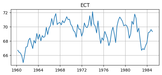
Error Correction Term#
Interpreting the cointegration coefficients, or the error correction term (ECT)
\[\begin{align*} ECT_{t-1} &= \hat{\beta}' [\tilde{y}_{t-1},\tilde{c}_{t-1}] = \tilde{y}_{t-1} - 0.94 \tilde{c}_{t-1} \\ \rightarrow \tilde{y}_{t-1} &= 0.94 \tilde{c}_{t-1} + ECT_{t-1} \end{align*}\]The long-run linear relationship between GDP and consumption is strongly positive, \(\tilde{y}_t \approx 0.94 \tilde{c}_t\), and the ECT measures how far away the system is from equilibrium.
\(\hat{\alpha}_1 = -0.24\) (and is significant) measures how much GDP corrects disequilibrium, i.e., returns to equilibrium
The significance indicates which variables adjust, e.g., \(\hat{\alpha}_2\) was not significant so consumption probably does not correct disquilibrium.
The sign indicates the direction of adjustment of each variable towards the long-run equilibrium, e.g., since \(\hat{\alpha}_1 < 0\), GDP pushes the system back to equilibrium
The magnitude is the speed or strength of adjustment, e.g., since \(|\hat{\alpha}_1| > |\hat{\alpha}_2|\), GDP adjusts more quickly than consumption.
# Error Correction Term
ECT = sample_lev@results_vecm.beta
ECT.name = 'ECT'
# Plot data
fig, ax = plt.subplots(figsize=(6.5,2.5))
ax.plot(ECT); ax.grid(); ax.set_title(ECT.name);
# Unit Root Test
test = adf_test(ECT,'c')
display(test)
| ECT | |
|---|---|
| Test Statistic | -3.330790 |
| p-value | 0.013557 |
| # of Lags | 11.000000 |
| # of Obs | 88.000000 |
Result: reject that the ECT has a unit root and conclude that it is probably stationary, as desired.
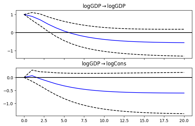
Impulse Response Functions#
The estimated VECM cannot be used to compute IRFs
IRFs are only defined for a VAR with stationary time series or a VAR with cointegrated time series in levels (e.g., Christiano et al., 2005)
Instead we would estimate a reduced form VAR(\(p\)) separately to compute IRFs, where \(p\) comes from the selected lag order from the VECM estimation
Then we can ask the question, how much does an increase in income change consumption and for how long?
Since both GDP and consumption are both clearly endogenous to many other things in the macroeconomy, it doesn’t make sense to use a Cholesky decomposition (e.g., orthogonalization) to estimate shocks.
# VAR model
from statsmodels.tsa.api import VAR
# make the VAR model
model_var = VAR(sample_lev)
# Estimate VAR(p)
results_var = model_var.fit(model_vecm.k_ar_diff + 1)
# Assign impulse response functions (IRFs)
irf = results_var.irf(20)
# Plot IRFs
fig = irf.plot(orth=False,impulse='logGDP',figsize=(6.5,4));
fig.suptitle(" ");
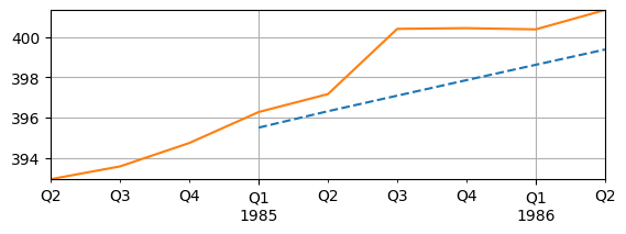
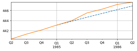
Forecasting#
With the estimated VAR, forecasts can also be made
Want to compare forecasts to actual data
This may not be a great example because the 1980s is still relative volatile
# Lag order and end of sample
p = results_var.k_ar
last_obs = sample_lev.values[-p:]
# Forecast 6 quarters ahead
h = 6;
forecast = results_var.forecast(y=last_obs, steps=h)
forecast_df = pd.DataFrame(forecast, columns=sample_lev.columns)
dates = pd.date_range(start='03-31-1985', periods=h, freq='QE')
forecast_df.index = dates  # Assign to index
# Actual Data
start_date = pd.Timestamp('12-31-1984')-pd.DateOffset(months=3*p)
end_date = pd.Timestamp('12-31-1984')+pd.DateOffset(months=3*h)
print(f'start date = {start_date}, end date = {end_date}')
sample_forecast = data[start_date:end_date]
start date = 1984-06-30 00:00:00, end date = 1986-06-30 00:00:00
fig, ax = plt.subplots(figsize=(6.5,2))
forecast_df['logGDP'].plot(ax=ax, linestyle='--')
sample_forecast['logGDP'].plot(ax=ax, linestyle='-')
ax.grid(); ax.autoscale(tight=True);
fig, ax = plt.subplots(figsize=(6.5,2))
forecast_df['logCons'].plot(ax=ax, linestyle='--')
sample_forecast['logCons'].plot(ax=ax, linestyle='-')
ax.grid(); ax.autoscale(tight=True);