AR Model

by Professor Throckmorton
for Time Series Econometrics
W&M ECON 408/PUBP 616
Slides

AR(\(p\)) Model

• The AR(\(p\)) model is: \(y_t = \phi_1 y_{t-1} + \phi_2 y_{t-2} + \dots + \phi_p y_{t-p} + \varepsilon_t\)

• \(\phi_1\), \(\phi_2\), \(\ldots\), \(\phi_p\) are the autoregressive parameters that quantify the influence of past values on the current value

• \(\varepsilon_t\) is white noise error term (or innovation) with mean zero and constant variance, \(\sigma^2\)

AR(\(1\)) Model

• An AR(\(1\)) Model is a special case of the AR(\(p\))

  \[ y_t = \phi y_{t-1} + \varepsilon_t \]

• An AR(\(1\)) is often used to model cyclical dynamics

• e.g., the fluctuations in an AR(1) series where \(\phi = 0.95\) appear much more persistent (i.e., smoother) than those where \(\phi = 0.4\)

AR(\(1\)) for any mean

• An AR(\(1\)) model is covariance stationary if \(|\phi| < 1\)

• Suppose \(E[y_t] = E[y_{t-1}] \equiv \bar{y}\)

• Then \(E[y_t] = 0\) since \(E[y_t] = \phi E[y_{t-1}] + E[\varepsilon_t] \rightarrow (1-\phi)\bar{y} = 0 \rightarrow \bar{y} = 0\)

• Instead consider the AR(1) model with a generic mean: \(y_t - \mu = \phi(y_{t-1} - \mu) + \varepsilon_t\)

• Then \(E[y_t] = \mu\) since

  \[\begin{align*} E[y_t] - \mu &= \phi E[y_{t-1}] -\phi\mu + E[\varepsilon_t] \\ \rightarrow (1-\phi)\bar{y} &= (1-\phi)\mu \\ \rightarrow \bar{y} &= \mu \end{align*}\]

• You can rearrange the (any mean) AR(1) model as \(y_t = (1-\phi)\mu + \phi y_{t-1} + \varepsilon_t\)

AR(1) as MA(\(\infty\))

• The AR(1) model structure is the same at all points in time

  \[\begin{align*} y_t &= \phi y_{t-1} + \varepsilon_t \\ y_{t-1} &= \phi y_{t-2} + \varepsilon_{t-1} \\ y_{t-2} &= \phi y_{t-3} + \varepsilon_{t-2} \end{align*}\]

• Combine, i.e., recursively substitute, to get \(y_t = \phi^3 y_{t-3} + \phi^2 \varepsilon_{t-2}+ \phi \varepsilon_{t-1} + \varepsilon_t\)

• Rinse and repeat to get \(y_t = \sum_{i=0}^\infty \phi^i \varepsilon_{t-i}\) (i.e., the MA(\(\infty\)) Model or Wold Representation)

• And an MA(\(\infty\)) is invertible back to an AR(\(1\)) so long as \(|\phi| < 1\).

• An AR model that can be written as an MA(\(\infty\)) is causal (or exhibits causality).

• That property differentiates it from an invertible MA model, which can be expressed as an AR(\(\infty\)) model.

Variance

• Suppose \(\mu=0\) without loss of generality.

• Given \(Var(\varepsilon_t) = \sigma^2\) and \(|\phi| < 1\), then \(\gamma(0) \equiv Var(y_t)\)

  \[\begin{align*} &= Var\left(\sum_{i=0}^\infty \phi^i \varepsilon_{t-i}\right) \\ &= Var(\varepsilon_t + \phi \varepsilon_{t-1} + \phi^2 \varepsilon_{t-2} + \phi^3 \varepsilon_{t-3} + \phi^4 \varepsilon_{t-4} + \cdots) \\ &= \sigma^2 + \phi^2 \sigma^2 + (\phi^2)^2 \sigma^2 + (\phi^3)^2 \sigma^2 + (\phi^4)^2 \sigma^2 + \cdots \\ &= \sigma^2(1 + \phi^2 + (\phi^2)^2 + (\phi^2)^3 + (\phi^2)^4 + \cdots ) \\ &= \sigma^2/(1-\phi^2) \end{align*}\]

  See Geometric Series.

• \(Std(y_t) = \sqrt{\sigma^2/(1-\phi^2)}\)

Autocorrelation

• \(\gamma(1) = E[y_t y_{t-1}]\)

  \[\begin{align*} &= E[(\phi y_{t-1} + \varepsilon_t)y_{t-1}] \\ &= E[\phi y_{t-1}^2] + E[\varepsilon_t y_{t-1}] \\ &= \phi Var[y_{t-1}] + 0 \\ &= \phi \gamma(0) \\ &= \phi \sigma^2/(1-\phi^2) \end{align*}\]

• \(\rho(1) = \gamma(1)/\gamma(0) = \phi\)

• \(\gamma(2) = E[y_t y_{t-2}] = E[(\phi^2y_{t-2} + \varepsilon_t + \phi \varepsilon_{t-1})y_{t-2}] = \phi^2 E[y_{t-2}^2] = \phi^2 \gamma(0)\)

• \(\rho(2) \equiv \gamma(2)/\gamma(0) = \phi^2\)

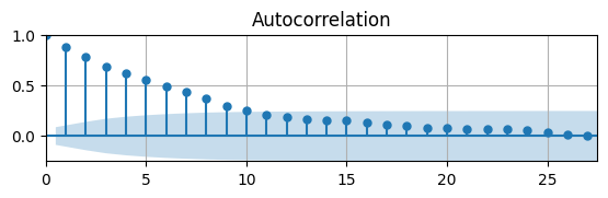
• In general, \(\rho(k) = \phi^k\), which is a very nice looking ACF.

• Thus, for an AR(\(1\)) process/model we can refer to \(\phi\) as the autocorrelation (AC) parameter/coefficient.

AR Model as DGP

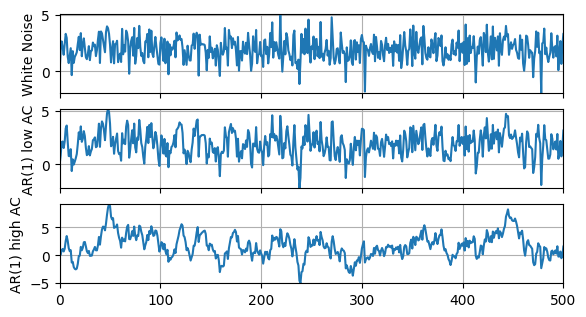
Let’s compare a couple different AR models to their underlying white noise.

1. White noise:

   \[ y_t = \mu + \varepsilon_t \]

2. AR(1), low AC:

   \[ y_t = (1-\phi_l)\mu + \phi_l y_{t-1} + \varepsilon_t \]

3. AR(1), high AC:

   \[ y_t = (1-\phi_h)\mu + \phi_h y_{t-1} + \varepsilon_t \]

# Libraries
import numpy as np
# Assign parameters
T = 501; mu = 2; phi_l = 0.5; phi_h = 0.9;
# Draw random numbers
rng = np.random.default_rng(seed=0)
eps = rng.standard_normal(T)
# Simulate time series
y = np.zeros([T,3])
for t in range(1,T):
    y[t,0] = mu + eps[t]
    y[t,1] = (1-phi_l)*mu + phi_l*y[t-1,1] + eps[t]
    y[t,2] = (1-phi_h)*mu + phi_h*y[t-1,2] + eps[t]

# Libraries
import pandas as pd
# Convert to DataFrame and plot
df = pd.DataFrame(y)
df.columns = ['White Noise','AR(1) low AC','AR(1) high AC']

# libraries
import matplotlib.pyplot as plt
# Plot variables
fig, axs = plt.subplots(len(df.columns),figsize=(6.5,3.5))
for idx, ax in enumerate(axs.flat):
    col = df.columns[idx]; y = df[col]
    ax.plot(y); ax.set_ylabel(col)
    ax.grid(); ax.autoscale(tight=True); ax.label_outer()
    print(f'{col}: \
E(y) = {y.mean():.2f}, Std(y) = {y.std():.2f}, \
AC(y) = {y.corr(y.shift(1)):.2f}')

White Noise: E(y) = 1.97, Std(y) = 1.02, AC(y) = -0.02
AR(1) low AC: E(y) = 1.94, Std(y) = 1.16, AC(y) = 0.48
AR(1) high AC: E(y) = 1.72, Std(y) = 2.18, AC(y) = 0.88

# Auto-correlation function
from statsmodels.graphics.tsaplots import plot_acf as acf
# Plot Autocorrelation Function
fig, ax = plt.subplots(figsize=(6.5,1.5))
acf(df['AR(1) high AC'],ax)
ax.grid(); ax.autoscale(tight=True);

# ARIMA model
from statsmodels.tsa.arima.model import ARIMA
# Define model
mod = ARIMA(df['AR(1) high AC'],order=(1,0,0))
# Estimate model
res = mod.fit()
summary = res.summary()
# Print summary tables
tab0 = summary.tables[0].as_html()
tab1 = summary.tables[1].as_html()
tab2 = summary.tables[2].as_html()
# print(tab0); print(tab1); print(tab2)

Estimation Results

Dep. Variable:	AR(1) high AC	No. Observations:	501
Model:	ARIMA(1, 0, 0)	Log Likelihood	-718.607

	coef	std err	z	P>|z|	[0.025	0.975]
const	1.6774	0.390	4.302	0.000	0.913	2.442
ar.L1	0.8843	0.021	41.211	0.000	0.842	0.926
sigma2	1.0282	0.059	17.442	0.000	0.913	1.144

Heteroskedasticity (H):	1.14	Skew:	-0.15
Prob(H) (two-sided):	0.41	Kurtosis:	3.45

• Parameter estimates are close to DGP and significantly different from \(0\)

• Residuals have skewness near \(0\) and kurtosis near \(3\) so they are probably normally distributed

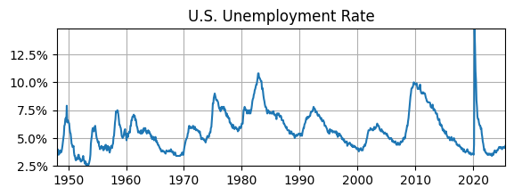
Modeling UR as AR(\(1\))

• The U.S. unemployment rate is very persistent.

• What if we model it with an AR(1)?

# Libraries
from fredapi import Fred
import pandas as pd
# Read Data
fred_api_key = pd.read_csv('fred_api_key.txt', header=None)
fred = Fred(api_key=fred_api_key.iloc[0,0])
data = fred.get_series('UNRATE').to_frame(name='UR')
data.index = pd.DatetimeIndex(data.UR.index.values,freq=data.UR.index.inferred_freq)
# Plot
fig, ax = plt.subplots(figsize=(6.5,2));
ax.plot(data.UR); ax.set_title('U.S. Unemployment Rate');
ax.yaxis.set_major_formatter('{x:,.1f}%')
ax.grid(); ax.autoscale(tight=True)

# Plot Autocorrelation Function
fig, ax = plt.subplots(figsize=(6.5,2.5))
acf(data.UR,ax);
ax.grid(); ax.autoscale(tight=True)

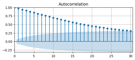
• The ACF decays very slow \(\rightarrow\) UR might be non-stationary.

• Let’s assume it is stationary for a moment and estimate an AR(\(1\)) model

# ARIMA model
from statsmodels.tsa.arima.model import ARIMA
# Define model
mod = ARIMA(data.UR,order=(1,0,0))
# Estimate model
res = mod.fit()
summary = res.summary()
# Print summary tables
tab0 = summary.tables[0].as_html()
tab1 = summary.tables[1].as_html()
tab2 = summary.tables[2].as_html()
#print(tab0); print(tab1); print(tab2)

Estimation Results

Dep. Variable:	VALUE	No. Observations:	925
Model:	ARIMA(1, 0, 0)	Log Likelihood	-496.551

	coef	std err	z	P>|z|	[0.025	0.975]
const	5.5470	0.761	7.289	0.000	4.055	7.039
ar.L1	0.9704	0.008	122.023	0.000	0.955	0.986
sigma2	0.1708	0.001	159.798	0.000	0.169	0.173

Heteroskedasticity (H):	6.35	Skew:	16.87
Prob(H) (two-sided):	0.00	Kurtosis:	428.90

• Estimate of AR coeffecient is very high at \(0.9704\), but the data is not a random walk

• Residuals are skewed and have excess kurtosis \(\rightarrow\) model is missing nonlinearity

Actual vs. Simulated Data

• What if we simulated data from AR(1) model setting the parameters to the previous estimates?

• What does a simulation from this estimated model look like?

# Assign parameters
T = len(data.UR); mu = 5.547; rho = 0.9704; sigma = np.sqrt(0.1708);
# Draw random numbers
rng = np.random.default_rng(seed=0)
eps = rng.standard_normal(T)
# Simulate time series
URsim = mu*np.ones([T,1])
for t in range(1,T):
    URsim[t,0] = (1-rho)*mu + rho*URsim[t-1,0] + sigma*eps[t];

# Plot Autocorrelation Function
fig, ax = plt.subplots(figsize=(6.5,1.5))
acf(URsim,ax)
ax.grid(); ax.autoscale(tight=True);

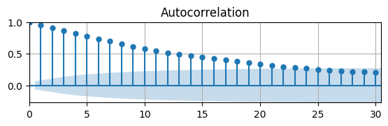
• This ACF approaches zero at shorter lags compared to the actual data.

• We know an AR(\(1\)) model with \(\phi = 0.9704\) generates stationary time series.

• Maybe the actual UR isn’t stationary?

# Add simulation to DataFrame
data['URsim'] = URsim
#  Variables to plot and ylabel
plotme = [['UR','Actual UR'],['URsim','Simulated UR']]
# Plot variables
fig, axs = plt.subplots(len(plotme),figsize=(6.5,3))
for idx, ax in enumerate(axs.flat):
    y = data[plotme[idx][0]]; ylabel = plotme[idx][1]
    ax.plot(y); ax.set_ylabel(ylabel)
    ax.yaxis.set_major_formatter('{x:.0f}%')
    ax.grid(); ax.autoscale(tight=True); ax.label_outer()
    print(f'{ylabel}: \
E(y) = {y.mean():.2f}, Std(y) = {y.std():.2f}, \
AC(y) = {y.corr(y.shift(1)):.2f}')

Actual UR: E(y) = 5.67, Std(y) = 1.71, AC(y) = 0.97
Simulated UR: E(y) = 5.21, Std(y) = 1.35, AC(y) = 0.95

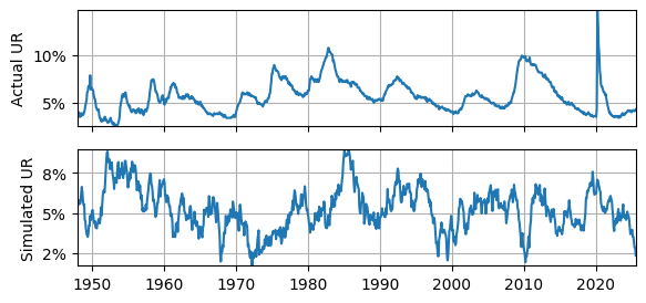
Does it fit?

• The actual UR is very smooth, but the AR(1) model is not.

• The simulated UR often falls below \(2\%\), whereas the actual UR does not.

• The actual UR meets or exceeds \(10\%\) a few times, whereas the simulated UR does not.

• The actual UR rises quickly and falls slowly, whereas the simulated UR seems to rise and fall at roughly the same rates.

• This all suggests that the AR(1) model is unable to reproduce some important features of the actual UR.

Partial ACF

• Most of the slides in this chapter are about the AR(\(1\)) model.

• Suppose the true DGP is an AR model, but we do not know the order.

• When the DGP is a MA model, we can use the ACF to determine the order since it drops off to zero after a certain lag.

• But for AR model, the autocorrelation at higher lags is influenced by the intermediate observations between \(t\) and \(t-k\), and even for an AR(\(1\)) model the ACF tapers slowly.

• Alternatively, Partial ACF (PACF) helps to identify the order of an AR model.

• The PACF at lag \(k\) is the correlation between \(y_t\) and \(y_{t-k}\) that is not explained by observations in between, \(\{y_{t-k+1}:y_{t-1}\}\)

• The PACF at lag \(k\) is denoted as \(\phi_{kk}\), and plotting \(\phi_{kk}\) against lag \(k\) forms the PACF plot.

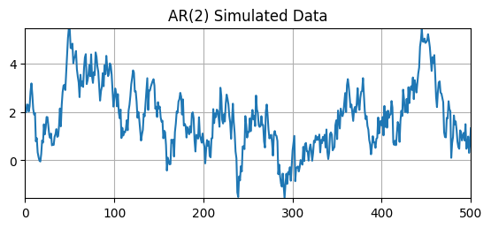
AR(\(2\)) Model

• Let’s simulate the following AR(\(2\)) model

  \[ y_t = (1-\phi_1-\phi_2)\mu + \phi_1 y_{t-1} + \phi_2 y_{t-2} + \sigma \varepsilon_t \]

  where \(\mu = 2\), \(\phi_1 = 0.8\), \(\phi_2 = 0.15\), and \(\sigma = 0.5\)

• We know the DGP and the true order of the AR model. Does the PACF suggest the same order?

# Assign parameters
T = 501; mu = 2; phi_1 = 0.8; phi_2 = 0.15; sigma = 0.5;
# Draw random numbers
rng = np.random.default_rng(seed=0)
eps = rng.standard_normal(T)
# Simulate time series
y = mu*np.ones([T,1])
for t in range(2,T):
    y[t,0] = (1-phi_1-phi_2)*mu + phi_1*y[t-1,0] + phi_2*y[t-2,0] + sigma*eps[t]

# Convert to DataFrame and plot
df = pd.DataFrame(y)
fig, ax = plt.subplots(figsize=(6.5,2.5))
ax.plot(df); ax.set_title('AR(2) Simulated Data')
ax.grid(); ax.autoscale(tight=True)

# Partial auto-correlation function
from statsmodels.graphics.tsaplots import plot_pacf as pacf
# Plot Autocorrelation Function
fig, ax = plt.subplots(figsize=(6.5,1.5))
pacf(df,ax)
ax.grid(); ax.autoscale(tight=True);

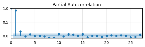
• The PACF is significantly different from zero for \(k = \{1,2\}\), which indicates the DGP is probably an AR(\(2\)).

• So the PACF is good at deterimining order so long as AR coefficients are large enough.

Modeling UR as AR(\(2\))

• Is a higher order AR model a good fit for the U.S. unemployment rate?

• Let’s first plot the PACF of the UR to see if we can determine an order.

# Plot Autocorrelation Function
fig, ax = plt.subplots(figsize=(6.5,1.5))
pacf(data.UR,ax);
ax.grid(); ax.autoscale(tight=True)

This suggests that an AR(1) might be the best model.

• What if we ignore the PACF and estimate an AR(2) anyway?

# Define model
mod = ARIMA(data.UR,order=(2,0,0))
# Estimate model
res = mod.fit()
summary = res.summary()
# Print summary tables
tab0 = summary.tables[0].as_html()
tab1 = summary.tables[1].as_html()
tab2 = summary.tables[2].as_html()
#print(tab0); print(tab1); print(tab2)

Estimation Results

Dep. Variable:	VALUE	No. Observations:	925
Model:	ARIMA(2, 0, 0)	Log Likelihood	-495.314

	coef	std err	z	P>|z|	[0.025	0.975]
const	5.5611	0.740	7.510	0.000	4.110	7.012
ar.L1	1.0208	0.009	109.007	0.000	1.002	1.039
ar.L2	-0.0517	0.010	-5.057	0.000	-0.072	-0.032
sigma2	0.1703	0.001	143.540	0.000	0.168	0.173

Heteroskedasticity (H):	6.37	Skew:	16.65
Prob(H) (two-sided):	0.00	Kurtosis:	423.48

• Both AR coefficients are significantly different from \(0\)

• But the AR(2) is still linear, i.e., normal and symmetric, so the residuals are still skewed and fat-tailed

• PACF did not help to determine that second lag might improve fit

UR First Difference

# Year-over-year growth rate
dUR = data.UR.diff(1); dUR = dUR.dropna()
# Plot
fig, ax = plt.subplots(figsize=(6.5,1.5));
ax.plot(dUR); ax.set_title('Change in U.S. Unemployment Rate (month to month)');
ax.yaxis.set_major_formatter('{x:,.0f}pp'); ax.grid(); ax.autoscale(tight=True)

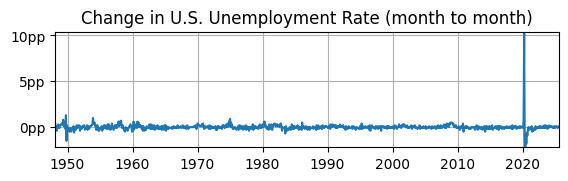
Is it stationary?

• Yes, mean looks constant around \(0\).

• Yes, volatility looks constant, except for COVID.

• Maybe not, it’s impossible to see if the autocovariance is constant.

# Plot Autocorrelation Function
fig, ax = plt.subplots(figsize=(6.5,1.5))
acf(dUR,ax)
ax.grid(); ax.autoscale(tight=True);

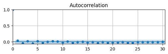
• The ACF indicates that the series is probably stationary.

• What does the PACF say?

# Plot Autocorrelation Function
fig, ax = plt.subplots(figsize=(6.5,1.5))
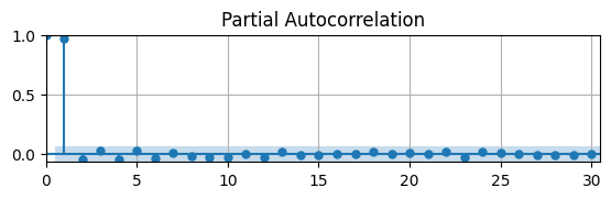
pacf(dUR,ax);
ax.grid(); ax.autoscale(tight=True)

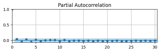
• The PACF shows that the autocorrelation is not significantly different from zero for all lags.

• What is the best model to estimate? Let’s try MA(\(1\)) and AR(\(1\)) and compare.

Estimation Results

# Define model
mod0 = ARIMA(dUR,order=(0,0,1))
mod1 = ARIMA(dUR,order=(1,0,0))
# Estimate model
res = mod1.fit(); summary = res.summary()
# Print summary tables
tab0 = summary.tables[0].as_html()
tab1 = summary.tables[1].as_html()
tab2 = summary.tables[2].as_html()
#print(tab0); print(tab1); print(tab2)

Dep. Variable:	VALUE	No. Observations:	924
Model:	ARIMA(0, 0, 1)	Log Likelihood	-500.699

	coef	std err	z	P>|z|	[0.025	0.975]
const	0.0007	0.025	0.027	0.979	-0.047	0.049
ma.L1	0.0398	0.008	4.893	0.000	0.024	0.056
sigma2	0.1731	0.001	185.366	0.000	0.171	0.175

Heteroskedasticity (H):	6.54	Skew:	16.40
Prob(H) (two-sided):	0.00	Kurtosis:	419.10

• The MA coefficient estimate is statistically significantly different from \(0\).

• However, the residuals are still probably heteroskedastic and not normally distributed.

• Thus, a linear/normal model is probably not the best choice.

Dep. Variable:	VALUE	No. Observations:	924
Model:	ARIMA(1, 0, 0)	Log Likelihood	-500.757

	coef	std err	z	P>|z|	[0.025	0.975]
const	0.0007	0.025	0.026	0.979	-0.048	0.049
ar.L1	0.0363	0.008	4.344	0.000	0.020	0.053
sigma2	0.1731	0.001	185.413	0.000	0.171	0.175

Heteroskedasticity (H):	6.55	Skew:	16.42
Prob(H) (two-sided):	0.00	Kurtosis:	419.51

• The AR coefficient is small/weak but estimate is statistically significantly different from \(0\).

• Like the MA(\(1\)) model, the residuals are still probably heteroskedastic and not normally distributed.

• This again confirms that a linear/normal model is probably not the best choice.