VAR Example Oil#
by Professor Throckmorton
for Time Series Econometrics
W&M ECON 408/PUBP 616
VAR#
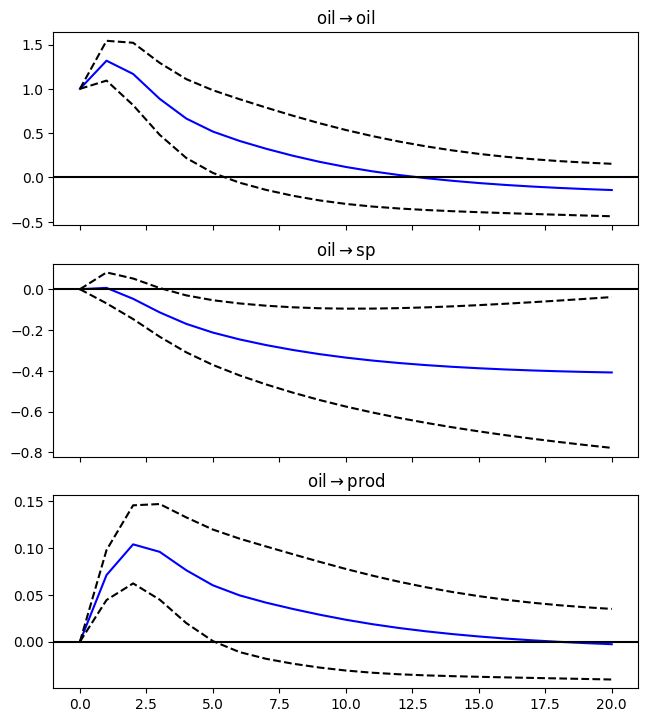
Big oil price increases are often associated with declines in production and asset prices. Read data on the price of crude oil (WTISPLC), industrial production (INDPRO), the S&P 500 (SP500), and the core consumer price index (CPILFESL).
# Libraries
from fredapi import Fred
import pandas as pd
# Setup acccess to FRED
fred_api_key = pd.read_csv('fred_api_key.txt', header=None).iloc[0,0]
fred = Fred(api_key=fred_api_key)
# Series to get
series = ['WTISPLC','INDPRO','SP500','CPILFESL']
rename = ['oil','prod','sp','price']
# Get and append data to list
dl = []
for idx, string in enumerate(series):
    var = fred.get_series(string).to_frame(name=rename[idx])
    dl.append(var)
    print(var.head(2)); print(var.tail(2))
             oil
1946-01-01  1.17
1946-02-01  1.17
              oil
2025-08-01  64.86
2025-09-01  63.96
              prod
1919-01-01  4.8654
1919-02-01  4.6504
                prod
2025-07-01  103.8194
2025-08-01  103.9203
                 sp
2015-10-29  2089.41
2015-10-30  2079.36
                 sp
2025-10-27  6875.16
2025-10-28  6890.89
            price
1957-01-01   28.5
1957-02-01   28.6
              price
2025-08-01  329.793
2025-09-01  330.542
# Concatenate data to create data frame (time-series table)
raw = pd.concat(dl, axis=1).sort_index()
# Make all columns numeric
raw = raw.apply(pd.to_numeric, errors='coerce')
# Resample/reindex to quarterly frequency
raw = raw.resample('ME').mean().dropna()
# Display dataframe
display(raw)
| oil | prod | sp | price | |
|---|---|---|---|---|
| 2015-10-31 | 46.22 | 100.1563 | 2084.385000 | 243.768 |
| 2015-11-30 | 42.44 | 99.4366 | 2080.616500 | 244.241 |
| 2015-12-31 | 37.19 | 98.9471 | 2054.079545 | 244.547 |
| 2016-01-31 | 31.68 | 99.4391 | 1918.597895 | 244.955 |
| 2016-02-29 | 30.32 | 98.9232 | 1904.418500 | 245.510 |
| ... | ... | ... | ... | ... |
| 2025-04-30 | 63.54 | 103.6224 | 5369.495714 | 326.430 |
| 2025-05-31 | 62.17 | 103.6570 | 5810.919524 | 326.854 |
| 2025-06-30 | 68.17 | 104.2115 | 6029.951500 | 327.600 |
| 2025-07-31 | 68.39 | 103.8194 | 6296.498182 | 328.656 |
| 2025-08-31 | 64.86 | 103.9203 | 6408.949524 | 329.793 |
119 rows × 4 columns
# Scientific computing
import numpy as np
data = pd.DataFrame()
# log real oil price
data['oil'] = 100*(np.log(raw['oil']/raw['price']))
# log real SP500
data['sp'] = 100*(np.log(raw['sp']/raw['price']))
# log industrial production
data['prod'] = 100*np.log(raw['prod'])
# Sample
sample = data['04-30-2015':'12-31-2024']
display(sample)
| oil | sp | prod | |
|---|---|---|---|
| 2015-10-31 | -166.280435 | 214.601217 | 460.673197 |
| 2015-11-30 | -175.006413 | 214.226408 | 459.952026 |
| 2015-12-31 | -188.336761 | 212.817560 | 459.458536 |
| 2016-01-31 | -204.538895 | 205.827541 | 459.954540 |
| 2016-02-29 | -209.153012 | 204.859431 | 459.434379 |
| ... | ... | ... | ... |
| 2024-08-31 | -142.817683 | 284.071677 | 463.491926 |
| 2024-09-30 | -151.900902 | 286.338423 | 463.079310 |
| 2024-10-31 | -149.705491 | 289.070597 | 462.706670 |
| 2024-11-30 | -152.869136 | 291.129327 | 462.448544 |
| 2024-12-31 | -152.836025 | 292.276288 | 463.516287 |
111 rows × 3 columns
# Johansen Cointegration Test
from statsmodels.tsa.vector_ar.vecm import coint_johansen
test = coint_johansen(sample, det_order=-1, k_ar_diff=2)
test_stats = test.lr1; crit_vals = test.cvt[:, 1]
# Print results
for r_0, (test_stat, crit_val) in enumerate(zip(test_stats, crit_vals)):
    print(f'H_0: r <= {r_0}')
    print(f'  Test Stat. = {test_stat:.2f}, 5% Crit. Value = {crit_val:.2f}')
    if test_stat > crit_val:
        print('  => Reject null hypothesis.')
    else:
        print('  => Fail to reject null hypothesis.')
H_0: r <= 0
  Test Stat. = 20.88, 5% Crit. Value = 24.28
  => Fail to reject null hypothesis.
H_0: r <= 1
  Test Stat. = 3.35, 5% Crit. Value = 12.32
  => Fail to reject null hypothesis.
H_0: r <= 2
  Test Stat. = 0.19, 5% Crit. Value = 4.13
  => Fail to reject null hypothesis.
# Select number of lags in VECM
from statsmodels.tsa.vector_ar.vecm import select_order
lag_order_results = select_order(
    sample, maxlags=8, deterministic='co')
print(f'Selected lag order (AIC) = {lag_order_results.aic}')
Selected lag order (AIC) = 1
# VAR model
from statsmodels.tsa.api import VAR
# make the VAR model
model = VAR(sample)
# Estimate VAR
results = model.fit(2)
# Assign impulse response functions (IRFs)
irf = results.irf(20)
# Plot IRFs
plt = irf.plot(orth=False,impulse='oil',figsize=(6.5,7.5));
plt.suptitle('');