ARIMA Model

by Professor Throckmorton
for Time Series Econometrics
W&M ECON 408/PUBP 616
Slides

Summary

• In a MA model, the current value is expressed as a function of current and lagged unobservable shocks.

• In an AR model, the current value is expressed as a function of its lagged values plus an unobservable shock.

• The general model is Autoregressive Integrated Moving Average Model, or ARIMA(\(p,d,q\)), of which MA are AR models are a special case.

• \((p,d,q)\) specifies the order for the autoregressive, integrated, and moving average components, respectively.

• Before we estimate ARIMA models, we should define the ARMA(\(p,q\)) model and the concept of integration.

ARMA Model

• An ARMA(\(p,q\)) model combines an AR(\(p\)) and MA(\(q\)) model:

  \[ y_t = \phi_0 + \phi_1 y_{t−1} + \cdots + \phi_p y_{t−p} + \varepsilon_t + \theta_1\varepsilon_{t-1} + \cdots + \theta_q\varepsilon_{t-q} \]

• As always, \(\varepsilon_t\) represents a white noise process with mean \(0\) and variance \(\sigma^2\).

• Stationarity: An ARMA(\(p,q\)) model is stationary if and only if its AR part is stationary (since all MA models produce stationary time series).

• Invertibility: An ARMA(\(p,q\)) model is invertible if and only if its MA part is invertible (since the AR model part is already in AR form).

• Causality: An ARMA(\(p, q\)) model is causal if and only if its AR part is causal, i.e., can be represented as an MA(\(\infty\)) model.

Key Aspects

• Model Building: Building an ARMA model involves plotting time series data, performing stationarity tests, selecting the order (\(p, q\)) of the model, estimating parameters, and diagnosing the model.

• Estimation Methods: Parameters in ARMA models can be estimated using methods such as conditional least squares and maximum likelihood.

• Order Determination: The order, (\(p, q\)), of an ARMA model can be determined using the ACF and PACF plots, or by using information criteria such as AIC, BIC, and HQIC.

• Forecasting: Covariance stationary ARMA processes can be converted to an infinite moving average for forecasting, but simpler methods are available for direct forecasting.

• Advantages: ARMA models can achieve high accuracy with parsimony. They often provide accurate approximations to the Wold representation with few parameters.

Integration

• The concept of integration in time series analysis relates to the stationarity of a differenced series.

• If a time series is integrated of order \(d\), \(I(d)\), it means that the time series needs to be differenced \(d\) times to become stationary.

• A time series that is \(I(0)\) is covariance stationary and does not need differencing.

• Differencing is a way to make a nonstationary time series stationary.

• An ARIMA(\(p,d,q\)) model is built by building an ARMA(\(p,q\)) model for the \(d\)th difference of the time series.

\(I(2)\) Example

# Libraries
from fredapi import Fred
import pandas as pd
# Read Data
fred_api_key = pd.read_csv('fred_api_key.txt', header=None)
fred = Fred(api_key=fred_api_key.iloc[0,0])
df = fred.get_series('CHNGDPNQDSMEI').to_frame(name='gdp')
df.index = pd.DatetimeIndex(df.index.values,freq=df.index.inferred_freq)
# Convert to billions of Yuan
df['gdp'] = df['gdp']/1e9
print(f'number of rows/quarters = {len(df)}')
print(df.head(2)); print(df.tail(2))

number of rows/quarters = 127
               gdp
1992-01-01  526.28
1992-04-01  648.43
                 gdp
2023-04-01  30803.76
2023-07-01  31999.23

# Plotting
import matplotlib.pyplot as plt
# Plot
fig, ax = plt.subplots(figsize=(6.5,2.5));
ax.plot(df.gdp);
ax.set_title('China Nominal GDP (Yuan)');
ax.yaxis.set_major_formatter('{x:,.0f}B')
ax.grid(); ax.autoscale(tight=True)

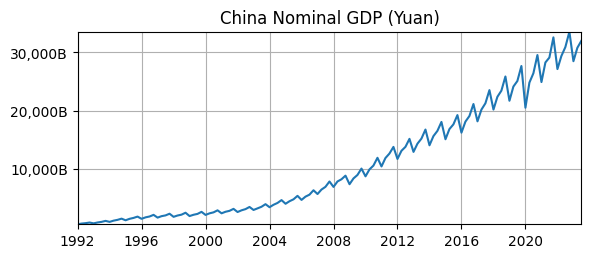
Is it stationary?

• No, there is an exponential time trend, i.e., the mean is not constant.

• No, the variance is smaller at the beginning that the end.

Seasonality

• We know that we can remove seaonality with a difference with lag \(4\).

• But we could also explicitly model seasonality as its own ARMA process.

• Let’s use the PACF to determine what the AR order of the seasonal component might be.

• First, let’s take \(\log\) to remove the exponential trend.

# Scientific computing
import numpy as np
# Remove expontential trend
df['loggdp'] = np.log(df['gdp'])

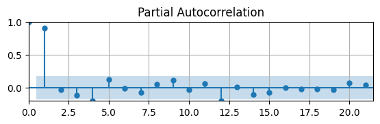
# Partial auto-correlation function
from statsmodels.graphics.tsaplots import plot_pacf as pacf
# Plot Autocorrelation Function
fig, ax = plt.subplots(figsize=(6.5,2))
pacf(df['loggdp'],ax); ax.grid(); ax.autoscale(tight=True)

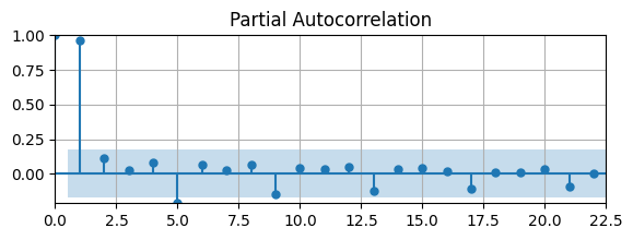
• PACF is significant at lags \(1\) and \(5\) (and also almost at lags \(9\), \(13\),…)

• i.e., this shows the high autocorrelation at a quarterly frequency

• You could model the seasonality as \(y_{s,t} = \phi_{s,0} + \phi_{s,4} y_{s,t-4} + \varepsilon_{s,t}\) (more on this later)

First Difference

# Year-over-year growth rate
df['d1loggdp'] = 100*(df['loggdp'] - df['loggdp'].shift(4))

# Plot
fig, ax = plt.subplots(figsize=(6.5,2));
ax.plot(df['d1loggdp']);
ax.set_title('China Nominal GDP Growth Rate (Year-over-year)');
ax.yaxis.set_major_formatter('{x:.0f}%')
ax.grid(); ax.autoscale(tight=True)

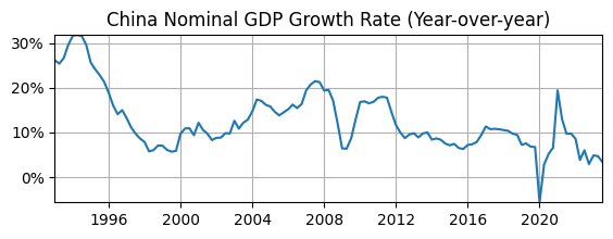
Does it look stationary?

• Maybe not, it might have a downward time trend.

• Maybe not, the volatility appears to change over time.

• Maybe not, the autocorrelation looks higher at the beginning than end of sample.

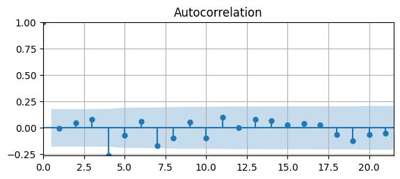
# Auto-correlation function
from statsmodels.graphics.tsaplots import plot_acf as acf
# Plot Autocorrelation Function
fig, ax = plt.subplots(figsize=(6.5,2))
acf(df['d1loggdp'].dropna(),ax)
ax.grid(); ax.autoscale(tight=True)

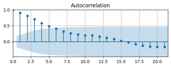
• The ACF tapers quickly, but starts to become non-zero for long lags.

• The AC is significantly different from zero for \(4\) lags. Let’s check the PACF to see if we can determine the order of an AR model.

# Plot Autocorrelation Function
fig, ax = plt.subplots(figsize=(6.5,1.5))
pacf(df['d1loggdp'].dropna(),ax)
ax.grid(); ax.autoscale(tight=True);

• The PACF suggests to estimate an AR(1) model.

• If we assume this first-differenced data is stationary and estimate an AR(1) model, what do we get?

# ARIMA model
from statsmodels.tsa.arima.model import ARIMA
# Define model
mod0 = ARIMA(df['d1loggdp'],order=(1,0,0))
# Estimate model
res = mod0.fit(); summary = res.summary()
# Print summary tables
tab0 = summary.tables[0].as_html(); tab1 = summary.tables[1].as_html(); tab2 = summary.tables[2].as_html()
#print(tab0); print(tab1); print(tab2)

Dep. Variable:	VALUE	No. Observations:	123
Model:	ARIMA(1, 0, 0)	Log Likelihood	-289.294

	coef	std err	z	P>|z|	[0.025	0.975]
const	12.9494	2.811	4.606	0.000	7.440	18.459
ar.L1	0.9399	0.026	36.315	0.000	0.889	0.991
sigma2	6.3511	0.348	18.243	0.000	5.669	7.033

Heteroskedasticity (H):	3.71	Skew:	0.11
Prob(H) (two-sided):	0.00	Kurtosis:	12.03

• The residuals might be heteroskedastic, i.e., their volatility varies over time.

• The kurtosis of the residuals indicate they are not normally distributed.

• That suggests that data might still be non-stationary and need to be differenced again.

Second Difference

# Second difference
df['d2loggdp'] = df['d1loggdp'] - df['d1loggdp'].shift(1)
# Plot
fig, ax = plt.subplots(figsize=(6.5,1.5));
ax.plot(df['d2loggdp']); ax.set_title('Difference of China Nominal GDP Growth Rate')
ax.yaxis.set_major_formatter('{x:.0f}pp')
ax.grid(); ax.autoscale(tight=True)

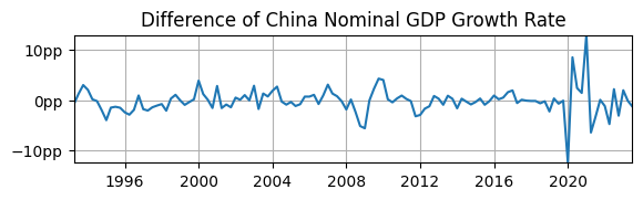
Does it look stationary?

• Yes, the sample mean appears to be \(0\).

• Yes, the volatility appears fairly constant over time, except during COVID.

• Yes, the autocorrelation also appears fairly constant over time, at least until COVID.

# Plot Autocorrelation Function
fig, ax = plt.subplots(figsize=(6.5,2.5))
acf(df['d2loggdp'].dropna(),ax)
ax.grid(); ax.autoscale(tight=True)

Estimation

# ARIMA model
from statsmodels.tsa.arima.model import ARIMA
# Define model
mod0 = ARIMA(df['loggdp'],order=(1,2,0))
mod1 = ARIMA(df['d1loggdp'],order=(1,1,0))
mod2 = ARIMA(df['d2loggdp'],order=(1,0,0))

# Estimate model
res = mod0.fit(); summary = res.summary()
# Print summary tables
tab0 = summary.tables[0].as_html(); tab1 = summary.tables[1].as_html(); tab2 = summary.tables[2].as_html()
#print(tab0); print(tab1); print(tab2)

Estimation Results ARIMA(\(1,2,0\))

Dep. Variable:	VALUE	No. Observations:	127
Model:	ARIMA(1, 2, 0)	Log Likelihood	49.700

	coef	std err	z	P>|z|	[0.025	0.975]
ar.L1	-0.6646	0.076	-8.722	0.000	-0.814	-0.515
sigma2	0.0263	0.004	6.541	0.000	0.018	0.034

Heteroskedasticity (H):	0.64	Skew:	-0.84
Prob(H) (two-sided):	0.15	Kurtosis:	2.35

• Warning: the AR coefficient estimate is negative!

• i.e., the way this time series has been differenced, the resulting series would flip from positive to negative every period.

• Why? ARIMA has taken the first difference at \(1\) lag, instead of lag \(4\), so the seasonality has not been removed.

Estimation Results ARIMA(\(1,1,0\))

Dep. Variable:	VALUE	No. Observations:	123
Model:	ARIMA(1, 1, 0)	Log Likelihood	-287.368

	coef	std err	z	P>|z|	[0.025	0.975]
ar.L1	0.0024	0.045	0.053	0.958	-0.087	0.091
sigma2	6.5086	0.361	18.042	0.000	5.802	7.216

Heteroskedasticity (H):	4.22	Skew:	0.32
Prob(H) (two-sided):	0.00	Kurtosis:	12.12

• AR coefficient estimate is not statistically significantly different from \(0\).

• That is consistent with the ACF plot, so AR(1) is model is not the best choice.

Estimation Results ARIMA(\(1, 0, 0\))

Dep. Variable:	VALUE	No. Observations:	122
Model:	ARIMA(1, 0, 0)	Log Likelihood	-287.042

	coef	std err	z	P>|z|	[0.025	0.975]
const	-0.1863	0.231	-0.806	0.420	-0.639	0.267
ar.L1	-0.0025	0.045	-0.055	0.956	-0.092	0.087
sigma2	6.4739	0.357	18.126	0.000	5.774	7.174

Heteroskedasticity (H):	4.34	Skew:	0.32
Prob(H) (two-sided):	0.00	Kurtosis:	12.10

• These results are nearly identical to estimating the ARIMA(\(1,1,0\)) with first-differenced data.

• i.e., once you remove seasonality, you can difference your data manually or have ARIMA do it for you.

ARIMA seasonal_order

• statsmodels ARIMA also has an argument to specify a model for seasonality.

• Above, a first difference at lag 4 removed the seasonality.

• seasonal_order=(P,D,Q,s) is the order of seasonal model for the AR parameters, differences, MA parameters, and periodicity (\(s\)) .

• We saw the periodicity of the seasonality in the data was \(4\) (and confirmed that with the PACF).

• Let’s model the seasonality as an ARIMA(\(1,1,0\)) (since the seasonal component is strongly autocorrelated and the data is integrated) with periodicity of \(4\).

• Then we can we estimate an ARIMA(\(1,1,0\)) using just \(\log(GDP)\)

mod3 = ARIMA(df['loggdp'],order=(1,1,0),seasonal_order=(1,1,0,4))
# Estimate model
res = mod3.fit(); summary = res.summary()
# Print summary tables
tab0 = summary.tables[0].as_html(); tab1 = summary.tables[1].as_html(); tab2 = summary.tables[2].as_html()
#tab0 = summary.tables[0].as_text(); tab1 = summary.tables[1].as_text(); tab2 = summary.tables[2].as_text()
#print(tab0); print(tab1); print(tab2)

Dep. Variable:	VALUE	No. Observations:	127
Model:	ARIMA(1, 1, 0)x(1, 1, 0, 4)	Log Likelihood	278.588

	coef	std err	z	P>|z|	[0.025	0.975]
ar.L1	0.0024	0.048	0.050	0.960	-0.092	0.096
ar.S.L4	-0.2598	0.043	-6.034	0.000	-0.344	-0.175
sigma2	0.0006	3.64e-05	16.652	0.000	0.001	0.001

Heteroskedasticity (H):	3.09	Skew:	-0.49
Prob(H) (two-sided):	0.00	Kurtosis:	10.65

• The estimates for the AR parameter is the same as estimating an ARIMA(1,1,0) with first-differenced \(\log(GDP)\) at lag \(4\).

• There is an additional AR parameter for the seasonal component ar.S.L4, i.e., we’ve controlled for the seasonality.

• While you can do this, it’s more transparent to remove seasonality by first differencing, then estimate an ARIMA model.

Unit Root(s)

• The presence of unit roots make time series non-stationary.

• Trend Stationarity: A trend-stationary time series has a deterministic time trend and is stationary after the trend is removed.

• Difference Stationarity: A difference-stationary time series has a stochastic time trend and becomes stationary after differencing.

• Unit root tests, e.g., the augmented Dickey-Fuller test (ADF test) are used to detect the presence of a unit root in a time series.

• Unit root tests help determine if differencing is required to achieve stationarity, suggesting a stochastic time trend.

• If an AR model has a unit root, it is called a unit root process, e.g., the random walk model.

AR(\(p\)) Polynomial

• Consider the AR(\(p\)) model: \(y_t = \phi_1 y_{t-1} + \phi_2 y_{t-2} + \dots + \phi_p y_{t-p} + \varepsilon_t\)

• Whether an AR(\(p\)) produces stationary time series depends on the parameters \(\phi_j\), e.g., for AR(\(1\)), \(|\phi_1|<1\)

• This can be written in terms of an AR polynomial with the lag operator, \(L\), defined as \(L^jy_t \equiv y_{t-j}\)

  \[ \varepsilon_t = y_t - \phi_1 y_{t-1} - \phi_2 y_{t-2} - \dots - \phi_p y_{t-p} = (1 - \phi_1 L - \phi_2 L^2 - \dots - \phi_p L^p)y_t \]

• Define the AR polynomial as \(\Phi(L) \equiv 1 - \phi_1 L - \phi_2 L^2 - \dots - \phi_p L^p\)

Unit Roots of AR(\(p\))

• To find the unit roots of an AR(\(p\)), set \(\Phi(r) = 0\) and solve for \(r\) (which is sometimes complex), and the number of roots will equal the order of the polynomial.

• An AR(\(p\)) has a unit root if the modulus of any of the roots equal \(1\).

• For each unit root, the data must differenced to make it stationary, e.g., if there are \(2\) unit roots then the data must be differenced twice.

• If the modulus of all the roots exceeds \(1\), then the AR(\(p\)) is stationary.

Examples

• AR(\(1\)): \(y_t = \phi_1 y_{t-1} + \varepsilon_t\)

  • \(\Phi(r) = 0 \rightarrow 1-\phi_1 r = 0 \rightarrow r = 1/\phi_1\)

  • Thus, an AR(\(1\)) has a unit root, \(r = 1\), if \(\phi_1 = 1\).

  • If \(\phi_1 = 1\), then \(y_t = y_{t-1} + \varepsilon_t\) is a random walk model that produces non-stationary time series.

  • But the first difference \(\Delta y_t = y_t - y_{t-1} = \varepsilon_t\) is stationary (since \(\varepsilon_t\) is white noise).

  • Note if \(|\phi_1| < 1\), then \(|r|>1\) and the AR(\(1\)) is stationary.

• AR(\(2\)): \(y_t = \phi_1 y_{t-1} + \phi_2 y_{t-2} + \varepsilon_t\) or \(\varepsilon_t = (1 - \phi_1 L - \phi_2 L^2) y_t\)

  • The AR(\(2\)) polynomial has a factorization such that \(1 - \phi_1 L - \phi_2 L^2 = (1-\lambda_1 L)(1-\lambda_2 L)\) with roots \(r_1 = 1/\lambda_1\) and \(r_2 = 1/\lambda_2\)

  • Thus, an AR(\(2\)) model is stationary if \(|\lambda_1| < 1\) and \(|\lambda_2| < 1\).

  • Given the mapping \(\phi_1 = \lambda_1 + \lambda_2\) and \(\phi_2 = -\lambda_1 \lambda_2\), we can prove that the modulus of both roots exceed \(1\) if

    • \(|\phi_2| < 1\)

    • \(\phi_2 + \phi_1 < 1\)

    • \(\phi_2 - \phi_1 < 1\)

Unit Root Test

• The augmented Dickey-Fuller test (ADF test) has hypotheses

  • \(h_0\): The time series has a unit root, indicating it is non-stationary.

  • \(h_A\): The time series does not have a unit root, suggesting it is stationary.

• Test Procedure

  • Write an AR(\(p\)) model with the AR polynomial, \(\Phi(L)y_t = \varepsilon_t\).

  • If the AR polynomial has a unit root, it can be written as \(\Phi(L) = \varphi(L)(1 - L)\) where \(\varphi(L) = 1 - \varphi_1 L - \cdots - \varphi_{p-1} L^{p-1}\).

  • Define \(\Delta y_t = (1 - L)y_t = y_t - y_{t-1}\).

  • An AR(\(p\)) model with a unit root is then \(\Phi(L)y_t = \varphi(L)(1 - L)y_t = \varphi(L)\Delta y_t = \varepsilon_t\).

  • Thus, testing \(\Phi(L)\) for a unit root is equivalent to the test \(h_0: \rho = 0\) vs. \(h_A: \rho < 0\) in

  \[ \Delta y_t = \rho y_{t-1} + \varphi_1 \Delta y_{t-1} + \cdots + \varphi_{p-1} \Delta y_{t-p+1} + \varepsilon_t \]

• Intuition: A stationary process reverts to its mean, so \(\Delta y_t\) should be negatively related to \(y_{t-1}\).

adfuller

• In statsmodels, the function adfuller() conducts an ADF unit root test.

• If the p-value is smaller than \(0.05\), then the series is probably stationary.

# ADF Test
from statsmodels.tsa.stattools import adfuller
# Function to organize ADF test results
def adf_test(data):
    keys = ['Test Statistic','p-value','# of Lags','# of Obs']
    values = adfuller(data)
    test = pd.DataFrame.from_dict(dict(zip(keys,values[0:4])),
                                  orient='index',columns=[data.name])
    return test

ADF test results

test = adf_test(df['d1loggdp'].dropna())
#print(test.to_markdown())

	d1loggdp
Test Statistic	-3.1799
p-value	0.0211781
# of Lags	4
# of Obs	118

• The p-value < \(0.05\), reject the null hypothesis that the process is non-stationary.

• The number of lags is chosen by minimizing the Akaike Information Criterion (AIC) (more on that soon).

dl = []
for column in df.columns:
    test = adf_test(df[column].dropna())
    dl.append(test)
results = pd.concat(dl, axis=1)
#print(results.to_markdown())

	gdp	loggdp	d1loggdp	d2loggdp
Test Statistic	4.294	-1.27023	-3.1799	-6.54055
p-value	1	0.642682	0.0211781	9.37063e-09
# of Lags	7	8	4	3
# of Obs	119	118	118	118

• China GDP has a unit root after taking log.

• China GDP is probably stationary after removing seasonality and converting to growth rate (p-value < \(0.05\)).

• Second difference of China GDP is almost certainly stationary.

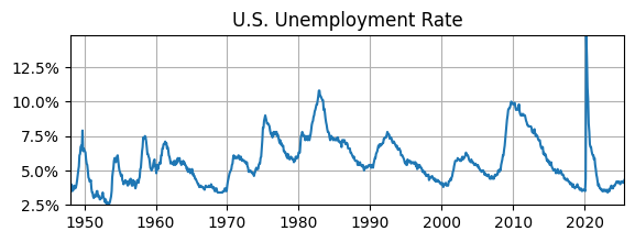
U.S. Unemployment Rate

# Read Data
fred_api_key = pd.read_csv('fred_api_key.txt', header=None)
fred = Fred(api_key=fred_api_key.iloc[0,0])
data = fred.get_series('UNRATE').to_frame(name='UR')
# Plot
fig, ax = plt.subplots(figsize=(6.5,2));
ax.plot(data.UR); ax.set_title('U.S. Unemployment Rate');
ax.yaxis.set_major_formatter('{x:,.1f}%')
ax.grid(); ax.autoscale(tight=True)

adf_UR = adf_test(data.UR)
print(adf_UR)

                        UR
Test Statistic   -3.926630
p-value           0.001847
# of Lags         1.000000
# of Obs        929.000000

• ADF test suggests that U.S. unemployment rate is stationary (p-value < 0.05).

• This doesn’t necessarily contradict the ACF, which suggested the UR might be non-stationary, i.e., we couldn’t tell with certainty.

• This result may not be surprising since modeling the UR as AR(\(1\)) led to an estimate of the AC parameter that was less than \(1\), i.e., it was not close to a random walk.

Order Determination

• There are a lot of possible choices for the orders of an ARIMA(\(p,d,q\)) model.

• Even if the data is not seasonal and already stationary, there are plenty of possibilities for an ARMA(\(p,q\)) model.

• In the ADF tests above, adfuller selected the \(p\) lags for an AR(\(p\)) model for the first-differenced time series to test for a unit root.

• How do we select the best orders for an ARMA(\(p,q\)) model?

Information Criterion

• Information criteria are used for order determination (i.e., model selection) of ARMA(\(p,q\)) models.

• In adfuller, the default method to select lags is the Akaike Information Criterion (AIC). Another choice is the Bayesian Information Criterion (BIC) (a.k.a. Schwarz Information Criterion (SIC)).

• The AIC and BIC are commonly used in economics research using time series data.

• But there are other choices as well, e.g., the Hannan-Quinn Information Criterion (HQIC).

• The goal of AIC, BIC, and HQIC is to estimate the out-of-sample mean square prediction error, so a smaller value indicates a better model.

AIC vs. BIC

• Let \(\mathcal{L}\) be the maximized log-likelihood of the model, \(K\) be the number of estimated parameters, and \(n\) be the sample size of the data.

  • \(AIC = -2 \mathcal{L} + 2 K\)

  • \(BIC = -2 \mathcal{L} + \log(n) K\)

• The key difference is that

  • AIC has a tendency to overestimate the model order.

  • BIC places a bigger penalty on model complexity, hence the best model is parsimonious relative to AIC.

• Consistency, i.e., as the sample size increases does the information criteria select the true model?

  • AIC is not consistent, but it is asymptotically efficient, which is relevant for forecasting (more on that much later).

  • BIC is consistent.

• When AIC and BIC suggest different choices, most people will choose the parsimonious model using the BIC.

Likelihood Function

• Likelihood function: Probability of the observed time series data given a model and its parameterization.

• Maximum Likelihood Estimation: For a given model, find the parameterization that maximizes the likelihood function, i.e., such that the observed time series has a higher probability than with any other parameterizaiton.

• The likelihood function is the joint probability distribution of all observations.

• In ARMA/ARIMA models, the likelihood function is just a product of Gaussian/normal distributions since that is the distribution of the errors/innovations.

• Order determination/model selection:

  • Given some time series data and a menu of models, which model has the highest likelihood and is relatively parsimonious?

  • e.g., for each AR model we can compute the ordinary least squares estimates and then the value of the likelihood function for that parameterization.

Example

• Assume an MA(2) model: \(y_t = \mu + \varepsilon_t + \theta_1 \varepsilon_{t-1} + \theta_2 \varepsilon_{t-2}\), where \(\varepsilon_t \sim \mathcal{N}(0, \sigma^2)\) are i.i.d. normal errors. Note: by construction \(y_t\) is uncorrelated with \(y_{t-3}\)

• The likelihood function is the joint probability distribution of the observations \(y_1, y_2, \dots, y_T\), given parameters of the model \(\Theta = \{\mu, \theta_1, \theta_2, \sigma^2\}\)

  \[ \mathcal{L}(\Theta| y_1, \dots, y_T) = \prod_{t=1}^{T} f(y_t | y_{t-1}, y_{t-2}; \Theta) \]

  where \(f(y_t | y_{t-1}, y_{t-2}; \Theta)\) is the conditional normal density

  \[ f(y_t | y_{t-1}, y_{t-2};\Theta) = \frac{1}{\sqrt{2\pi \sigma^2}} \exp\left( -\frac{\varepsilon_t^2}{2\sigma^2} \right) \]

• Combining the previous expressions and substituting out \(\varepsilon_t\) for \(y_t - \mu - \theta_1 \varepsilon_{t-1} - \theta_2 \varepsilon_{t-2}\) yields

  \[ \mathcal{L}(\Theta) = \prod_{t=1}^{T} \frac{1}{\sqrt{2\pi \sigma^2}} \exp\left( -\frac{(y_t - \mu - \theta_1 \varepsilon_{t-1} - \theta_2 \varepsilon_{t-2})^2}{2\sigma^2} \right) \]

• The log-likelihood function (i.e., taking natural log converts a product to a sum) is

  \[ \log \mathcal{L}(\Theta) = -\frac{T}{2} \log(2\pi\sigma^2) - \frac{1}{2\sigma^2} \sum_{t=1}^{T} (y_t - \mu - \theta_1 \varepsilon_{t-1} - \theta_2 \varepsilon_{t-2})^2 \]

• To estimate \(\mu, \theta_1, \theta_2, \sigma^2\), maximize this log-likelihood function, i.e., \(\hat{\Theta} = \textrm{arg max}_\Theta \log \mathcal{L}(\Theta)\).

• Because \(\log \mathcal{L}(\Theta)\) is nonlinear in the parameters, numerical methods such as nonlinear optimization or the conditional likelihood approach are used in practice.