VAR Example Oil - Time Series

by Professor Throckmorton
for Time Series Econometrics
W&M ECON 408

VAR¶

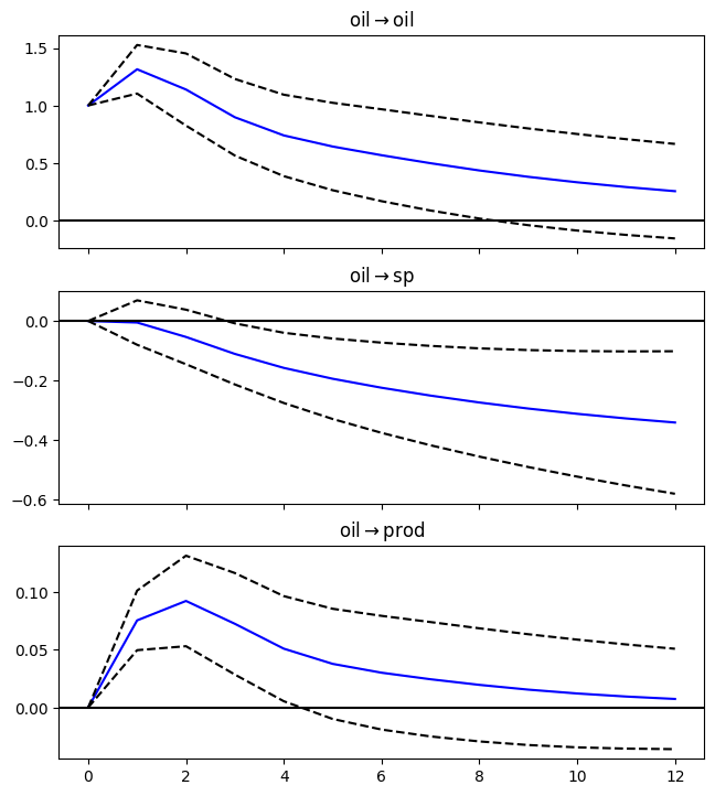
Big oil price increases are often associated with declines in production and asset prices. Read data on the price of crude oil (WTISPLC), industrial production (INDPRO), the S&P 500 (SP500), and the core consumer price index (CPILFESL).

# Libraries
from fredapi import Fred
import pandas as pd
# Setup access to FRED
fred_api_key = pd.read_csv('fred_api_key.txt', header=None).iloc[0,0]
fred = Fred(api_key=fred_api_key)
# Series to get
series = ['WTISPLC','INDPRO','SP500','CPILFESL']
rename = ['oil','prod','sp','price']
# Get and append data to list
dl = []
for idx, string in enumerate(series):
    var = fred.get_series(string).to_frame(name=rename[idx])
    dl.append(var)
    print(var.head(2)); print(var.tail(2))

             oil
1946-01-01  1.17
1946-02-01  1.17
              oil
2026-01-01  60.04
2026-02-01  64.51
              prod
1919-01-01  4.8739
1919-02-01  4.6585
                prod
2026-01-01  102.3963
2026-02-01  102.5510
                 sp
2016-03-24  2035.94
2016-03-25      NaN
                 sp
2026-03-20  6506.48
2026-03-23  6581.00
            price
1957-01-01   28.5
1957-02-01   28.6
              price
2026-01-01  332.793
2026-02-01  333.512

# Concatenate data to create data frame (time-series table)
raw = pd.concat(dl, axis=1).sort_index()
# Resample/reindex to quarterly frequency
raw = raw.resample('ME').mean().dropna()
# Display dataframe
display(raw)

/var/folders/dj/q2kc_rtn4kz50sd41yg6w8xc0000gq/T/ipykernel_36376/3185200006.py:2: Pandas4Warning: Sorting by default when concatenating all DatetimeIndex is deprecated.  In the future, pandas will respect the default of `sort=False`. Specify `sort=True` or `sort=False` to silence this message. If you see this warnings when not directly calling concat, report a bug to pandas.
  raw = pd.concat(dl, axis=1).sort_index()

# Scientific computing
import numpy as np
data = pd.DataFrame()
# log real oil price
data['oil'] = 100*(np.log(raw['oil']/raw['price']))
# log real SP500
data['sp'] = 100*(np.log(raw['sp']/raw['price']))
# log industrial production
data['prod'] = 100*np.log(raw['prod'])
# Sample
#sample = data['03-01-2021':'02-28-2026']
sample = data
display(sample)

# VAR model
from statsmodels.tsa.api import VAR
# make the VAR model
model = VAR(sample)

# Search over candidate lag lengths
lag_selection = model.select_order(maxlags=12)   # change 12 as needed
print(lag_selection.summary())

# BIC-selected lag
p = lag_selection.selected_orders['bic']
print("Selected lag by BIC:", p)

 VAR Order Selection (* highlights the minimums)  
==================================================
       AIC         BIC         FPE         HQIC   
--------------------------------------------------
0        14.26       14.34   1.564e+06       14.29
1        7.932       8.232       2785.       8.053
2       7.417*      7.942*      1665.*      7.630*
3        7.517       8.266       1842.       7.821
4        7.662       8.636       2133.       8.057
5        7.774       8.973       2395.       8.260
6        7.846       9.270       2586.       8.424
7        7.889       9.538       2717.       8.558
8        7.971       9.844       2973.       8.730
9        7.962       10.06       2979.       8.812
10       7.997       10.32       3128.       8.939
11       8.006       10.55       3212.       9.039
12       8.094       10.87       3579.       9.218
--------------------------------------------------
Selected lag by BIC: 2

/Users/vultureview/venv/myst-env/lib/python3.12/site-packages/statsmodels/tsa/base/tsa_model.py:473: ValueWarning: A date index has been provided, but it has no associated frequency information and so will be ignored when e.g. forecasting.
  self._init_dates(dates, freq)

# Estimate VAR
results = model.fit(p)
# Assign impulse response functions (IRFs)
irf = results.irf(12)
# Plot IRFs
plt = irf.plot(orth=False,impulse='oil',figsize=(6.5,7.5));
plt.suptitle('');