VAR Example Fed - Time Series

by Professor Throckmorton
for Time Series Econometrics
W&M ECON 408

Summary¶

Christiano et al. (2005): Christiano, Eichenbaum, and Evans “Nominal Rigidities and the Dynamic Effects of a Shock to Monetary Policy” (Journal of Polical Economy, 2005) has over 9,000 citations (astronomical!) according to google scholar.
Let $\mathbf{Y}_t$ denote variables observed between 1965Q3 to 1995Q3,
$\begin{gather*} \mathbf{Y}_t = [\mathbf{Y}_{1t}, R_t, \mathbf{Y}_{2t}]' \end{gather*}$
(1)
$\mathbf{Y}_{1t}$ : real GDP, real consumption, GDP deflator, real investment, real wages, and labor productivity
$R_t$ : federal funds rate
$\mathbf{Y}_{2t}$ : real profits, M2 growth rate

Assumptions¶

$R_t$ appears after $\mathbf{Y}_{1t}$ , i.e., the assumption is that none of the variables in $\mathbf{Y}_{1t}$ respond contemporaneously to $R_t$ , so the real economy lags behind monetary policy (citing Friedman)
“All these variables, except money growth, have been natural logged.”
“With one exception (the growth rate of money), all the variables in are included in levels.”
“The VAR contains four lags of each variable, and the sample period is 1965:3–1995:3.”

Read Data¶

# Libraries
from fredapi import Fred
import pandas as pd
# Setup access to FRED
fred_api_key = pd.read_csv('fred_api_key.txt', header=None)
fred = Fred(api_key=fred_api_key.iloc[0,0])
# Series to get
series = ['GDP','PCE','GDPDEF','GPDI','COMPRNFB','OPHNFB','FEDFUNDS','CP','M2SL']
rename = ['gdp','cons','price','inv','wage','prod','ffr','profit','money']
# Get and append data to list
dl = []
for idx, string in enumerate(series):
    var = fred.get_series(string).to_frame(name=rename[idx])
    dl.append(var)
    print(var.head(2)); print(var.tail(2))

            gdp
1946-01-01  NaN
1946-04-01  NaN
                  gdp
2025-07-01  31098.027
2025-10-01  31442.483
             cons
1959-01-01  306.1
1959-02-01  309.6
               cons
2025-12-01  21455.5
2026-01-01  21536.6
             price
1947-01-01  11.141
1947-04-01  11.299
              price
2025-07-01  129.430
2025-10-01  130.651
            inv
1939-01-01  NaN
1939-04-01  NaN
                 inv
2025-07-01  5419.029
2025-10-01  5516.971
              wage
1947-01-01  34.386
1947-04-01  34.670
               wage
2025-07-01  110.088
2025-10-01  111.082
              prod
1947-01-01  22.256
1947-04-01  22.762
               prod
2025-07-01  118.814
2025-10-01  119.338
             ffr
1954-07-01  0.80
1954-08-01  1.22
             ffr
2026-01-01  3.64
2026-02-01  3.64
            profit
1946-01-01     NaN
1946-04-01     NaN
              profit
2025-04-01  3355.897
2025-07-01  3591.344
            money
1959-01-01  286.6
1959-02-01  287.7
              money
2026-01-01  22469.1
2026-02-01  22667.3

# Concatenate data to create data frame (time-series table)
raw = pd.concat(dl, axis=1).sort_index()
# Resample/reindex to quarterly frequency
raw = raw.resample('QE').last().dropna()
# Display dataframe
display(raw)

/var/folders/dj/q2kc_rtn4kz50sd41yg6w8xc0000gq/T/ipykernel_91542/2474872120.py:2: Pandas4Warning: Sorting by default when concatenating all DatetimeIndex is deprecated.  In the future, pandas will respect the default of `sort=False`. Specify `sort=True` or `sort=False` to silence this message. If you see this warnings when not directly calling concat, report a bug to pandas.
  raw = pd.concat(dl, axis=1).sort_index()

Transform Data¶

# Scientific computing
import numpy as np
data = pd.DataFrame()
# log real GDP
data['gdp'] = 100*(np.log(raw['gdp']/raw['price']))
# log real Consumption
data['cons'] = 100*(np.log(raw['cons']/raw['price']))
# log price level
#data['price'] = 100*np.log(raw['price'])
data['inf'] = 400*(raw['price']/raw['price'].shift(1)-1)
# log real Investment
data['inv'] = 100*(np.log(raw['inv']/raw['price']))
# log real Wage
data['wage'] = 100*(np.log(raw['wage']/raw['price']))
# log labor productivity
data['prod'] = 100*np.log(raw['prod'])
# log federal funds rate
data['ffr'] = 100*np.log(raw['ffr'])
# log real Profits
data['profit'] = 100*(np.log(raw['profit']/raw['price']))
# M2 growth rate
data['money'] = 100*(raw['money']/raw['money'].shift(1)-1)

# Christiano et al. (2005) sample
sample = data['09-30-1965':'09-30-1995']
display(sample)

Non-stationarity¶

# Plotting
import matplotlib.pyplot as plt
# Plot GDP
fig, ax = plt.subplots(figsize=(6.5,2.5))
ax.plot(sample['gdp'])
ax.set_title('100 log(Real GDP)')
ax.grid()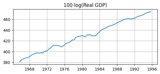

Q: Do these transformations make the data stationary? A: Clearly not.
Sims et al. (1990) find that VARs in levels can yield consistent impulse response functions even if the variables are non-stationary, I(1), and cointegrated.
Fortunately, Christiano et al. (2005) is only concerned with estimating IRFs.

Cointegration¶

Suppose you have two non-stationary time series: $y_t$ and $x_t$ , both I(1).
Typically, any linear combination of them, $z_t = y_t - \beta x_t$ , would also be non-stationary.
But if some linear combination is stationary, then the variables are cointegrated.
The coefficients (like $[1, -\beta]$ ) form a cointegrating vector.
This implies the variables share a stable long-run relationship despite short-run fluctuations.

Example¶

Let $y_t$ be $\log(GDP)$ (i.e., income) and $x_t$ be $\log(PCE)$ (i.e., consumption)
Both series are non-stationary, I(1), because they have a stochastic time trend.
There might exist a linear combination $z_t = y_t - \beta x_t$ that is stationary, I(0), meaning
- Income and consumption have a long-run linear relationship, i.e., they are cointegrated.
- Deviations from the long-run are mean-reverting.

Estimation¶

# VAR model
from statsmodels.tsa.api import VAR
# make the VAR model
model = VAR(sample)

# Estimate VAR(4)
results = model.fit(4)
# Assign impulse response functions (IRFs)
irf = results.irf(20)

# Plot IRFs
plt = irf.plot(orth=True,impulse='ffr',figsize=(6.5,22.5));
plt.suptitle('');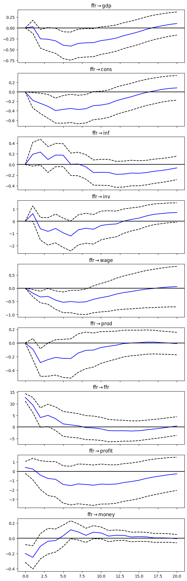

# Search over candidate lag lengths
lag_selection = model.select_order(maxlags=4)
print(lag_selection.summary())

# BIC-selected lag
p = lag_selection.selected_orders['bic']
print("Selected lag by BIC:", p)

 VAR Order Selection (* highlights the minimums) 
=================================================
      AIC         BIC         FPE         HQIC   
-------------------------------------------------
0       27.48       27.69   8.565e+11       27.56
1      4.550*      6.675*      95.03*      5.413*
2       4.597       8.634       101.8       6.236
3       4.966       10.92       156.2       7.381
4       5.273       13.13       238.7       8.465
-------------------------------------------------
Selected lag by BIC: 1

# Estimate VAR(4)
results = model.fit(p)
# Assign impulse response functions (IRFs)
irf = results.irf(20)

# Plot IRFs
plt = irf.plot(orth=True,impulse='ffr',figsize=(6.5,22.5));
plt.suptitle('');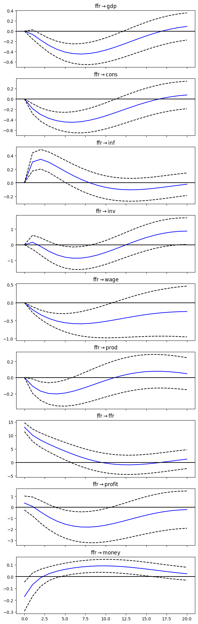

References¶

Christiano, L. J., Eichenbaum, M., & Evans, C. L. (2005). Nominal Rigidities and the Dynamic Effects of a Shock to Monetary Policy. Journal of Political Economy, 113(1), 1–45. https://doi.org/10.1086/426038
Sims, C. A., Stock, J. H., & Watson, M. W. (1990). Inference in linear time series models with some unit roots. Econometrica, 113–144. 10.2307/2938337