Money Market
by Professor Throckmorton
for Intermediate Macro
W&M ECON 304
Slides
Introduction
In the goods market, everything is real, and we would have to imagine that the output of firms is being bartered among households, i.e., there was no money.
Of course, money is essential to how a macroeconomy works, serving the essential purposes of a store of value, medium of exchange, and unit of account.
People need money to buy the goods, services, and assets that make up their consumption and savings.
However, money is not the best store of value since it does not earn interest.
Thus, we should think of households as portfolio managers that choose between assets with different uses.
Money and Bonds
It’s useful to compare assets across these dimensions:
Return
Liquidity
Risk
Money has no return, but bonds do.
Money is used for transactions, i.e., it is liquid. Some bonds with large volume markets issued by governments or corporations with excellent credit ratings are nearly as liquid, since buyers are abundant.
And bonds vary by risk depending on who issued them, whether they have good or bad credit ratings.
Let’s consider money vs. a bond with similar risk and liquidity, i.e., both originate from the U.S. government, where the only difference is their rate of return.
Portfolio Choice
Suppose households, or portfolio managers, allocate their financial portfolios between money and bonds.
The only difference is that bonds earn positive interest.
Q: How much of the portfolio should be allocated to bonds?
A: It depends on the interest rate. A higher interest rate makes bonds more appealing than a lower rate.
U.S. T-Bills
If the bonds are 3-month U.S. Treasury Bills (i.e., T-Bills), then they look a lot like a simple loan.
Consider a simple loan where the principal is and the interest rate is .
The borrower must pay back principal + interest or back to the lender.
When the U.S. Treasury (the borrower) issues T-Bills, they set the face value on the bond, which is paid to the bond holder (the lender) 3 months after the purchase.
When the U.S. Treasury auctions T-Bills, the price at which the market buys them essentially becomes the principal, i.e., how much the borrower initially receives.
Bond Pricing
Denote the bond’s face value as , the bond price at auction as , and the interest rate as , then
which has the same structure as a simple loan, principal loan payment.
This can be rearranged as
which says the price of a bond today is equal to present value future cash flow, which in this case is the bond’s face value.
Prediction: if higher demand for bonds drives the bond price up, then the interest rate (or yield) falls. I.e., a bond’s price is inversely related to its yield.
Money Demand
Money is useful for transactions, i.e., it’s liquid, and bonds are useful because they earn a positive return.
The opportunity cost of holding money then is the interest forgone from not holding bonds.
Thus, people should hold more money when the interest rate is low and more bonds when the interest rates are high.
The quantity of money demanded with respect to the interest rate satisfies the law of demand.
Money demand also depends on income. Higher household income would lead to more money demand (i.e., money is a normal good).
Source
import numpy as np
import matplotlib.pyplot as plt
x = np.linspace(0, 40, 100)
plt.figure(figsize=(5, 3))
# plot a downward sloping line
plt.plot(x, 40 - x)
# plot a downward sloping line
plt.plot(x, 20 - x)
# remove the x and y tick labels
plt.xticks([]); plt.yticks([]);
# label the x axis as Money (M) and the y axis as Interest Rate (i)
plt.xlabel('Money, M', loc='right')
plt.ylabel('Interest Rate, i', loc='top')
# add label to the line M^d
plt.text(39, 7, '$M^d(Y_{high})$', fontsize=10, verticalalignment='bottom', horizontalalignment='right');
# add label to bottom line M^d(Y_{low})
plt.text(39, -7, '$M^d(Y_{low})$', fontsize=10, verticalalignment='top', horizontalalignment='right');
# add arrow pointing right between the two money demand curves
plt.annotate('', xy=(23, 15), xytext=(10, 15),
             arrowprops=dict(arrowstyle='->', color='black', linewidth=1.5));
# add label below arrow "Increase in Y"
plt.text(17, 13, 'Increase in $Y$', fontsize=10, verticalalignment='top', horizontalalignment='center');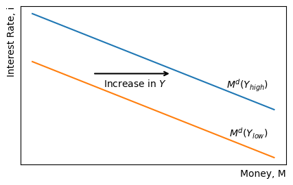
Money Supply
Money originates from a central bank.
Central bank asset purchases create high-powered money, e.g., reserves at member banks of the Federal Reserve System.
Banks use those reserves to make loans, which creates deposits that are part of the money supply.
In other words, one part of money creation is public due to central bank transactions, and the other part of money creation is private due to the lending behavior of banks.
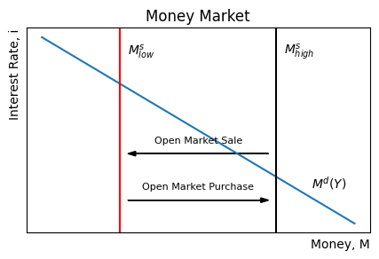
The Fed influences the money supply with open market operations
If the Fed buys bonds, then money is created (i.e., expansionary monetary policy).
If the Fed sells bonds, then money is destroyed (i.e., contractionary monetary policy).
Since modern central banking targets interest rates, we will assume that money supply is perfectly inelastic and the money supply is whatever it needs to be to achieve the desired interest rate.
Source
x = np.linspace(0, 40, 100)
plt.figure(figsize=(5, 3))
# plot a downward sloping line
plt.plot(x, 40 - x)
# add title "Money Market"
plt.title('Money Market')
# remove the x and y tick labels
plt.xticks([]); plt.yticks([]);
# label the x axis as Money (M) and the y axis as Interest Rate (i)
plt.xlabel('Money, M', loc='right')
plt.ylabel('Interest Rate, i', loc='top')
# add label to the line M^d
plt.text(39, 7, '$M^d(Y)$', fontsize=10, verticalalignment='bottom', horizontalalignment='right');
# add vertical line for money supply and label it M^s
plt.axvline(x=30, color='black')
plt.text(31, 35, '$M^s_{high}$', fontsize=10, verticalalignment='bottom', horizontalalignment='left');
# add vertical line for money supply and label it M^s
plt.axvline(x=10, color='red')
plt.text(11, 35, '$M^s_{low}$', fontsize=10, verticalalignment='bottom', horizontalalignment='left');
# add horizontal arrow pointing left from black vertical line to red vertical line
plt.arrow(29, 15, -17, 0, head_width=1, head_length=1, fc='black', ec='black');
# label arrow "Open Market Sale"
plt.text(20, 17, 'Open Market Sale', fontsize=8, verticalalignment='bottom', horizontalalignment='center');
# add horizontal arrow pointing right from red vertical line to black vertical line
plt.arrow(11, 5, 17, 0, head_width=1, head_length=1, fc='black', ec='black');
# label arrow "Open Market Purchase"
plt.text(20, 7, 'Open Market Purchase', fontsize=8, verticalalignment='bottom', horizontalalignment='center');
Equilibrium
Suppose the current interest rate is below equilibrium.
At that interest rate, there is a shortage of money.
Portfolio managers sell bonds to increase money in their portfolios.
As people sell bonds, the bond price falls and the interest rate (yield) rises.
As the interest rate rises, people are willing to hold less money.
Source
x = np.linspace(0, 40, 100)
plt.figure(figsize=(5, 3))
# plot a downward sloping line
plt.plot(x, 40 - x)
# add title "Money Market"
plt.title('Money Market')
# remove the x and y tick labels
plt.xticks([]); plt.yticks([]);
# label the x axis as Money (M) and the y axis as Interest Rate (i)
plt.xlabel('Money, M', loc='right')
plt.ylabel('i', loc='top', rotation=0)
# add label to the line M^d
plt.text(39, 7, '$M^d(Y)$', fontsize=10, verticalalignment='bottom', horizontalalignment='right');
# add vertical line for money supply and label it M^s
plt.axvline(x=20, color='black')
plt.text(21, 35, '$M^s$', fontsize=10, verticalalignment='bottom', horizontalalignment='left');
# add dot at intersection of money supply and money demand
plt.plot(20, 20, 'ko')
# put dashed horizontal line between vertical axis and aggregate expenditure line at X=5
plt.axhline(20, xmin=0, xmax=15/30, color='black', linewidth=0.5, ls='--')
# label vertical axis i^* at intersection of horizontal line and vertical axis
plt.text(-4, 20, '$i^*$', fontsize=10, verticalalignment='center', horizontalalignment='left');
# horiztonal dashed line between M^s and M^d at Y= 10
plt.axhline(10, xmin=0, xmax=22/30, color='black', linewidth=0.5, ls='--')
# label vertical axis i_{low} at bottom horizontal line
plt.text(-6, 10, '$i_{low}$', fontsize=10, verticalalignment='center', horizontalalignment='left');
# add horizontal double arrow between M^s and M^d at Y= 10
plt.annotate('', xy=(30, 10), xytext=(20, 10),
             arrowprops=dict(arrowstyle='<->', color='black', linewidth=1.5));
# label double arrow "Shortage"
plt.text(25, 6, 'Shortage', fontsize=10, verticalalignment='bottom', horizontalalignment='center');
# put an arrow pointing up along the money demand curve between i_{low} and i^*
plt.arrow(30, 12, -8, 8, head_width=1, head_length=1, fc='black', ec='black');
# add label sell bonds next to arrow
plt.text(26, 17, 'Sell Bonds', fontsize=8, verticalalignment='bottom', horizontalalignment='left');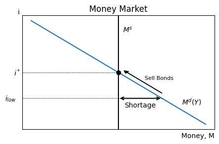
Monetary Policy
In modern central banking (since the 1990s), is whatever it needs to be to achieve a target interest rate in the short-run.
e.g., the Fed achieves their target interest rate with open market operations.
In the money market model, if money demand were to increase or decrease then the central bank should simultaneously change money supply to maintain their interest rate target.
Source
x = np.linspace(0, 60, 100)
plt.figure(figsize=(5, 3))
# plot a downward sloping line
plt.plot(x, 40 - x)
# add title "Money Market"
plt.title('Money Market')
# remove the x and y tick labels
plt.xticks([]); plt.yticks([]);
# label the x axis as Money (M) and the y axis as Interest Rate (i)
plt.xlabel('Money, M', loc='right')
plt.ylabel('i', loc='top', rotation=0)
# add label to the line M^d
plt.text(45, -10, '$M^d(Y_1)$', fontsize=10, verticalalignment='bottom', horizontalalignment='right');
# add vertical line for money supply and label it M^s
plt.axvline(x=10, color='black')
plt.text(11, 35, '$M^s_1$', fontsize=10, verticalalignment='bottom', horizontalalignment='left');
# add dot at intersection of money supply and money demand
plt.plot(10, 30, 'ko')
# put dashed horizontal line between vertical axis and aggregate expenditure line at X=5
plt.axhline(30, xmin=0, xmax=15/40, color='black', linewidth=0.5, ls='--')
# label vertical axis i^* at intersection of horizontal line and vertical axis
plt.text(-8, 30, '$i^*$', fontsize=10, verticalalignment='center', horizontalalignment='left');
# plot a downward sloping line
plt.plot(x + 20, 40 - x)
# add label to the line M^d
plt.text(65, -10, '$M^d(Y_2)$', fontsize=10, verticalalignment='bottom', horizontalalignment='right');
# add vertical line for money supply and label it M^s
plt.axvline(x=30, color='black')
plt.text(31, 35, '$M^s_3$', fontsize=10, verticalalignment='bottom', horizontalalignment='left');
# add dot at intersection of money supply and money demand
plt.plot(30, 30, 'ko')
# add right arrow between money demand curves
plt.annotate('', xy=(53, 5), xytext=(38, 5), arrowprops=dict(arrowstyle='->', color='black'));
# label the arrow between the money demand curves "1"
plt.text(45, 6, '2', fontsize=10, verticalalignment='bottom', horizontalalignment='center');
# add right arrow between both vertical lines
plt.annotate('', xy=(30, 5), xytext=(10, 5), arrowprops=dict(arrowstyle='->', color='black'));
# label the arrow between the money supply lines "2"
plt.text(20, 6, '3', fontsize=10, verticalalignment='bottom', horizontalalignment='center');
# label the left equilibrium point "0"
plt.text(7, 27, '1', fontsize=10, verticalalignment='center', horizontalalignment='center');
# label the right equilibrium point "2"
plt.text(27, 27, '3', fontsize=10, verticalalignment='center', horizontalalignment='center');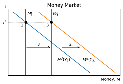
Suppose the central bank targets and the money market is in an initial equilibrium.
(For some reason) from to .
Money demand shifts right because it increases with income.
At , and there is a shortage of money.
Portfolio managers would sell bonds, the bond price would fall, and the interest would rise, except then it would no longer be at its target.
Thus, the central bank increases the money supply with open market purchases of bonds to maintain , i.e., they eliminate the shortage of money.