Macro Data

by Professor Throckmorton
for Intermediate Macro
W&M ECON 304
Slides

Gross Domestic Product (GDP)¶

• Gross Domestic Product (GDP) can be measured using

  • Value added approach

  • Expenditure approach

  • Income approach

• To illustrate these different approaches, consider a fictional island economy with a coconut farm, a restaurant, households, and a government

• The following example is borrowed from Williamson, Macroeconomics (6th Edition, 2018), Chapter 2, Pages 39-44

Coconut Farm

• Produces 10 million coconuts which are sold for $2 each

• Pays wages of $5 million to its workers

• Pays $0.5 million in interest on a loan

• Pays $1.5 million in taxes to the government

• Of the 10 million coconuts produced, 6 million go to the restaurant and 4 million are bought by consumers

Restaurant

• Earns $30 million in revenues during the year

• Faces intermediate input costs of $12 million

• Pays its workers $4 million in wages

• Pays the government $3 million in taxes

Government

• Collect taxes in order to provide national defense

• Uses all tax revenues to pay wages to the army

• Total taxes collected are $5.5 million

  • $4.5 million from producers

  • $1 million from households

Households

• Work for the producers and for the government, earning total wages of $14.5 million.

• Receive $0.5 million in interest from the producer

• Receive after-tax profits of $24 million from the producers (because some households own/manage the coconut farm and restaurant)

• Pay $1 million in taxes to the government

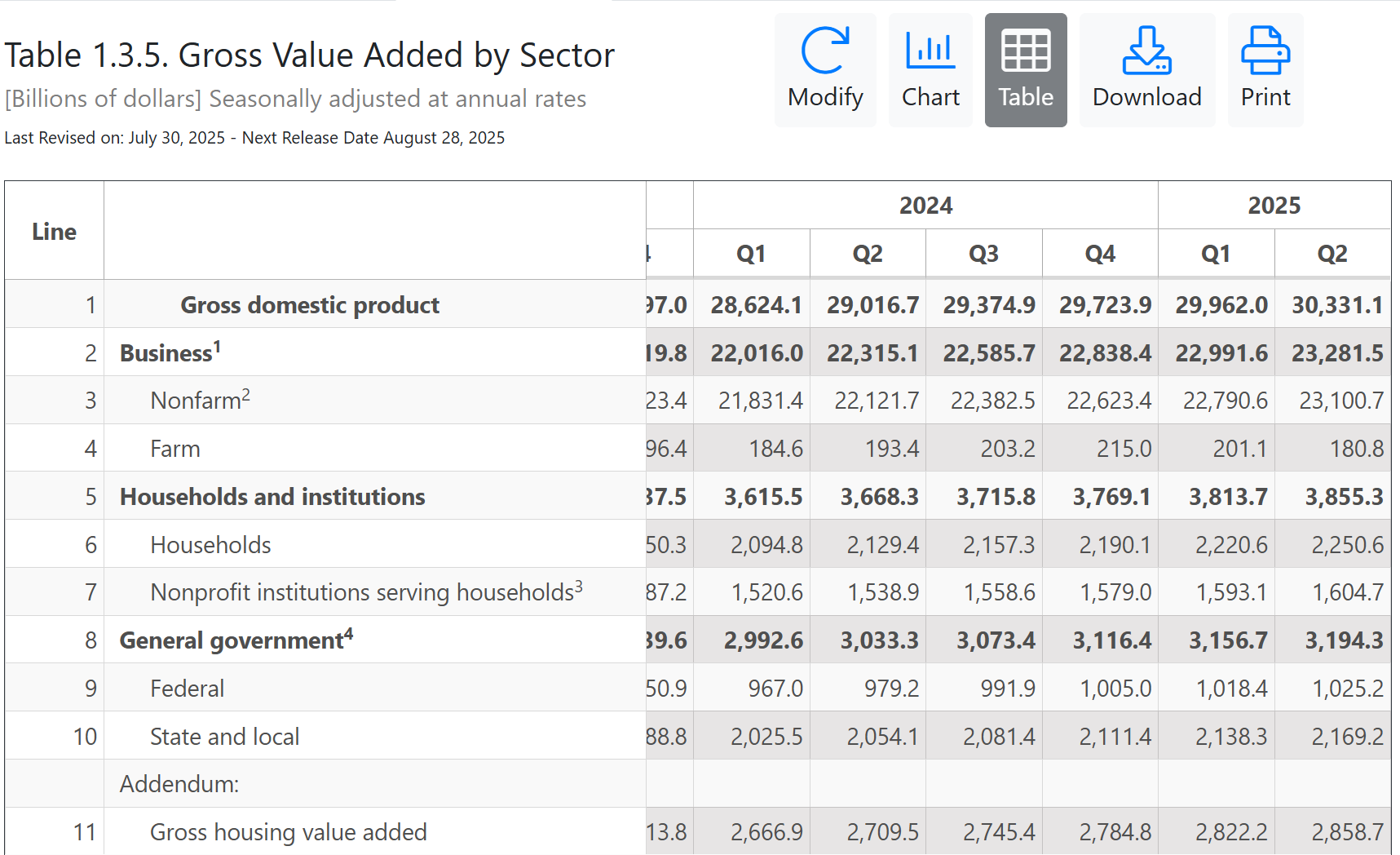
Value-Added Approach¶

• GDP is calculated as the sum of value added by labor to goods and services across all productive units in the economy.

• To calculate GDP using this approach, add the value of all final goods and services produced in the economy and then subtract the value of all intermediate goods used in production.

• Note that since national defense services provided by the government are not sold at market prices, it is standard practice to value these services at the cost of inputs to production.

• For actual data using the value added approach, see BEA, National Data, NIPA, Section 1, Tables 1.3.1-1.3.6

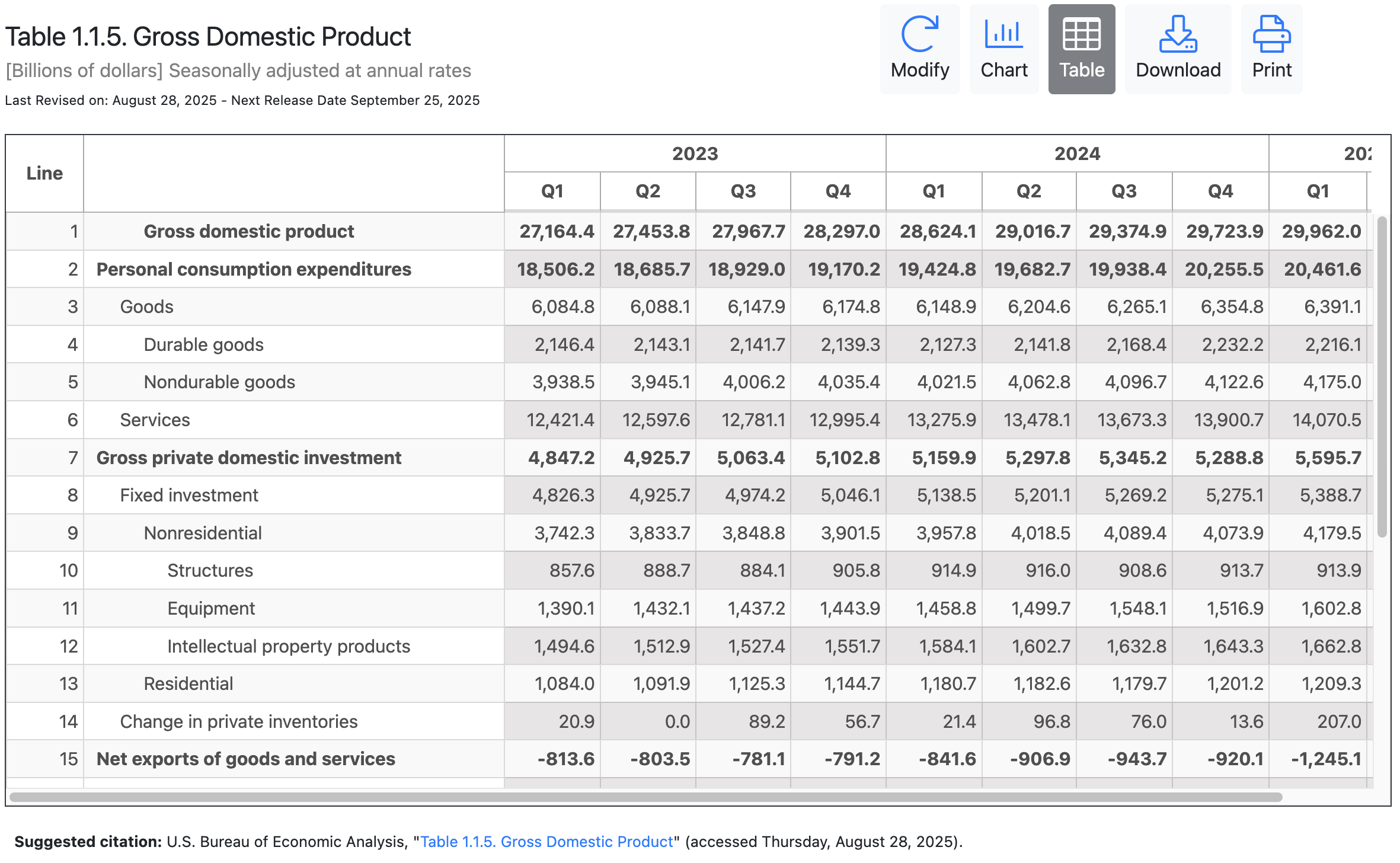
Expenditure Approach¶

• Calculate GDP as total spending on all final goods and services produced in the economy

• Again, do not count spending on intermediate goods and services

  $$\begin{align*} \mathrm{GDP}&= C+I+G+NX \\ &= (\$8~\mathrm{mil.}+\$30~\mathrm{mil.})+0+\$5.5~\mathrm{mil.}+0\\ &= \$43.5~\mathrm{million} \end{align*}$$

  (2)

• For actual data using the expenditure approach, see BEA, National Data, NIPA, Section 1, Tables 1.1.5-1.1.6

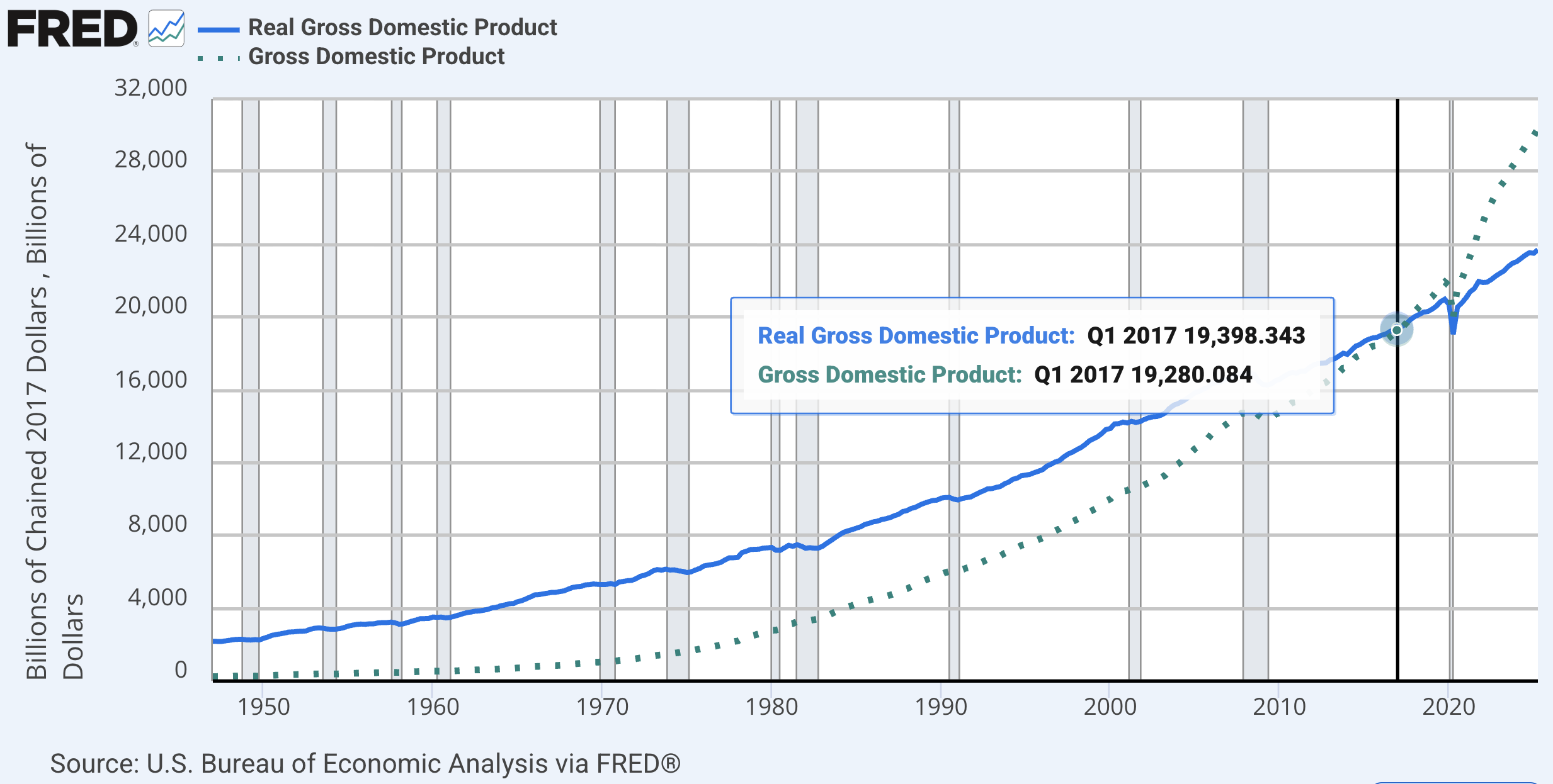
• You may also view GDP and its component as time series data on https://fred.stlouisfed.org/

• Search for “GDP”. Nominal GDP has the key “GDP” and real GDP has the key “GDPC1”.

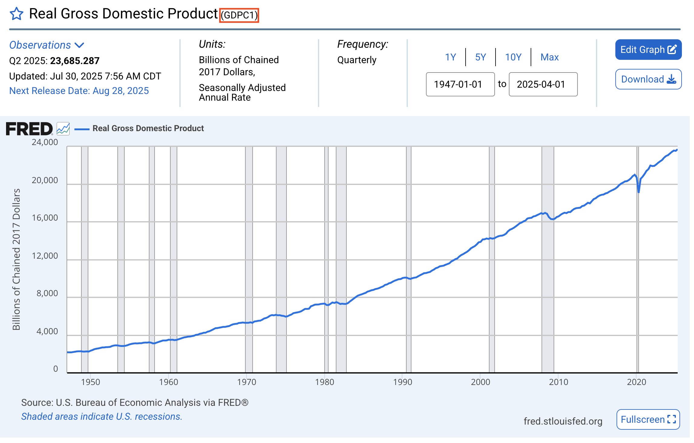
• The notebook, FRED, also creates this graph.

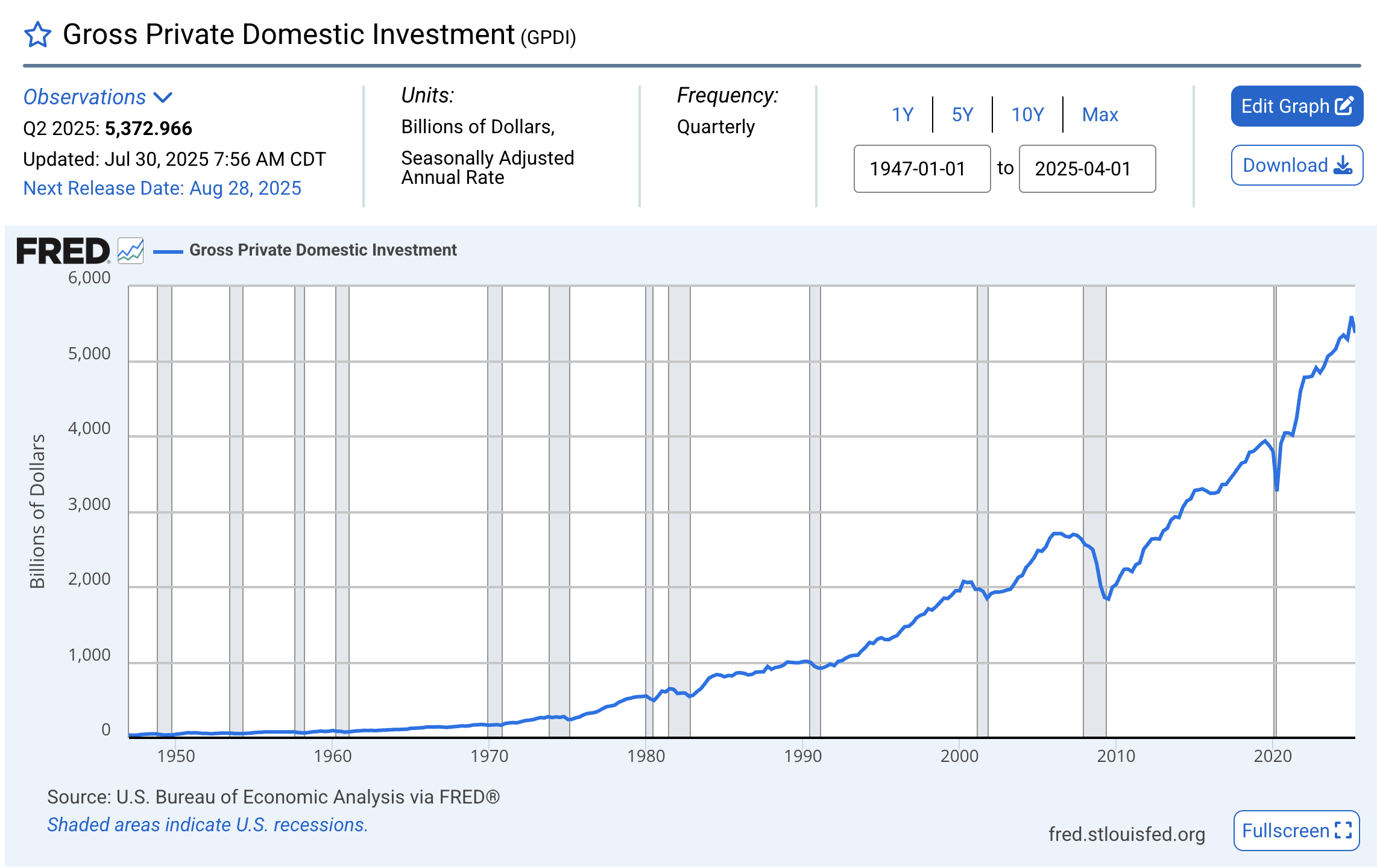
• Gross Private Domestic Investment has key “GPDI”

Income Approach¶

• To calculate GDP using this approach, add up all income received by economic agents contributing to production

• Income includes: profits made by firms, compensation of employees, rental income, net interest, taxes, and depreciation

  $$\begin{align*} \mathrm{GDP} &= \textrm{Wages}+\textrm{After-Tax Profits}+\textrm{Interest}+\textrm{Taxes} \\ &= \$14.5~\mathrm{mil.}+24~\mathrm{mil.}+0.5~\mathrm{mil.}+4.5~\mathrm{mil.}\\ &= \$43.5~\mathrm{million} \end{align*}$$

  (3)

• For actual data using the income approach, see BEA, National Data, NIPA, Section 2, Tables 2.1

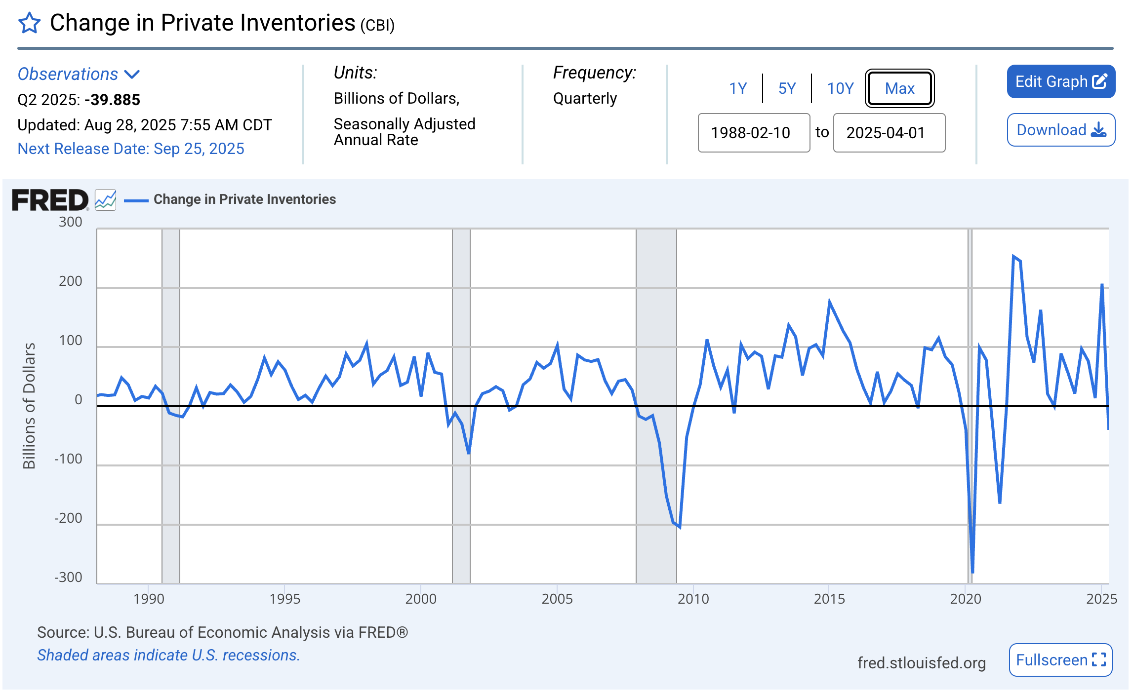
Inventory Investment¶

• What if the coconut farm produces 13 million coconuts instead of 10 million?

• Assume the extra 3 million units are stored as inventory

Three Approaches

• Value-Added Approach

  $$\begin{align*} \mathrm{GDP}&= \$26~\mathrm{mil.}+ (\$30~\mathrm{mil.}- \$12~\mathrm{mil.})+\$5.5~\mathrm{mil.}\\ &= \$49.5~\mathrm{million} \end{align*}$$

  (4)

• Expenditure Approach

  $$\begin{align*} \mathrm{GDP}&= C+I+G+NX \\ &= \$38~\mathrm{mil.}+\$6~\mathrm{mil.}+\$5.5~\mathrm{mil.}+0\\ &= \$49.5~\mathrm{million} \end{align*}$$

  (5)

• Income Approach

• Change in Private Inventories has key “CBI”

International Trade¶

• What if the restaurant imports 2 million coconuts at $2 each (in addition to the coconuts purchased domestically)?

• Assume the restaurant still sells $30 million in restaurant food to domestic consumers

• Thus, after-tax profits fall by $4 million.

Three Approaches

• Value-Added Approach

  $$\begin{align*} \mathrm{GDP}&= \$20~\mathrm{mil.}+ (\$30~\mathrm{mil.}- \$16~\mathrm{mil.})+\$5.5~\mathrm{mil.}\\ &= \$39.5~\mathrm{million} \end{align*}$$

  (7)

• Expenditure Approach

  $$\begin{align*} \mathrm{GDP}&= C+I+G+NX \\ &= \$38~\mathrm{mil.}+0+\$5.5~\mathrm{mil.}-\$4~\mathrm{mil.}\\ &= \$39.5~\mathrm{million} \end{align*}$$

  (8)

• Income Approach

  $$\begin{align*} \mathrm{GDP}&= \textrm{Wages}+\textrm{After-Tax Profits}+\textrm{Interest}+\textrm{Taxes} \\ &= \$14.5~\mathrm{mil.}+20~\mathrm{mil.}+0.5~\mathrm{mil.}+4.5~\mathrm{mil.}\\ &= \$39.5~\mathrm{million} \end{align*}$$

  (9)

Nominal and Real GDP¶

• Consider an economy where the only goods that are produced are apples and oranges

Quantities

Prices

Nominal GDP¶

• Year 1 Nominal GDP ($\$Y_1$) is

  $$\begin{align*} \$Y_1&=P_1^aQ_1^a+P_1^oQ_1^o\\ &=(\$1.00\times50)+(\$0.80\times100)\\ &=\$130 \end{align*}$$

  (10)

• Year 2 Nominal GDP ($\$Y_2$) is

  $$\begin{align*} \$Y_2&=P_2^aQ_2^a+P_2^oQ_2^o\\ &=(\$1.25\times80)+(\$1.60\times120)\\ &=\$292 \end{align*}$$

  (11)

• Percentage Increase

  $$\begin{align*} \frac{\$Y_2-\$Y_1}{\$Y_1}\times 100=\left(\frac{\$Y_2}{\$Y_1}-1\right)\times 100=125\% \end{align*}$$

  (12)

Real GDP¶

• Nominal GDP increases over time because:

  • The production of most goods increases over time

  • The prices of most goods also increase over time.

• Real GDP is constructed as the sum of the quantities of final goods multiplied by constant (rather than current) prices.

Real GDP: Year 1 Base Year

• Year 1 Real GDP with the base year (BY) in year 1 ($Y_1^1$)

  $$\begin{align*} Y_1^1=\$Y_1=\$130 \end{align*}$$

  (13)

• Year 2 Real GDP with the base year (BY) in year 1 ($Y_2^1$)

  $$\begin{align*} Y_2^1&=P_1^aQ_2^a+P_1^oQ_2^o\\ &=(\$1.00\times80)+(\$0.80\times120)\\ &=\$176 \end{align*}$$

  (14)

• Ratio of Real GDP in Year 2 to Real GDP in Year 1 ($g_1$), gross growth rate

  $$\begin{align*} g_1\equiv \frac{Y_2^1}{Y_1^1}=1.354 \end{align*}$$

  (15)

Real GDP: Year 2 Base Year

• Year 1 Real GDP with the base year (BY) in year 2 ($Y_1^2$)

  $$\begin{align*} Y_1^2&=P_2^aQ_1^a+P_2^oQ_1^o\\ &=(\$1.25\times50)+(\$1.60\times100)\\ &=\$222.50 \end{align*}$$

  (16)

• Year 2 Real GDP with the base year (BY) in year 2 ($Y_2^2$)

  $$\begin{align*} Y_2^2&=\$Y_2=\$292 \end{align*}$$

  (17)

• Ratio of Real GDP in Year 2 to Real GDP in Year 1 ($g_2$), gross growth rate:

  $$\begin{align*} g_2\equiv \frac{Y_2^2}{Y_1^2}=1.312 \end{align*}$$

  (18)

Base Year Effects

• Notice that the choice of the base year matters for the calculation of GDP

• Reason: Relative prices of the goods changed over time

  $$\begin{align*} \textrm{Year 1}=\frac{\$1.00}{\$0.80}=1.25\quad \textrm{Year 2}=\frac{\$1.25}{\$1.60}=0.78 \end{align*}$$

  (19)

• Had relative prices remained constant, the base would not have mattered

Chain-Weighted GDP¶

• The chain weighted ratio of real GDP in year 1 to real GDP in year 2 is

  $$\begin{align*} g_c\equiv \sqrt{g_1\times g_2}=\sqrt{1.354\times 1.312}=1.333 \end{align*}$$

  (20)

  a geometric average of the two ratios calculated above.

• The percentage growth rate in real GDP from year 1 to year 2 using the chain-weighted method is 33.33%

• Real GDP in Year 2 (in Year 1 dollars) is

  $$\begin{align*} \$Y_1\times g_c=\$130\times 1.33= \$173.29 \end{align*}$$

  (21)

• Real GDP in Year 1 (in Year 2 dollars) is

  $$\begin{align*} \frac{\$Y_2}{g_c}=\frac{\$292}{1.33}= \$219.05 \end{align*}$$

  (22)

Chain Weighting: Final Thoughts

• Notice that the growth rate in GDP between Year 1 and Year 2 is now identical whether we use Year 1 or Year 2 dollars

• For every two consecutive years, we use the chain-weighting method to calculate the growth rate in real GDP, and then use the growth rate to calculate real GDP. Real GDP is therefore “chained” together from one year to the next.

Unemployment Rate¶

• Employment ($N$) is the number of people who have a job

• Unemployment ($U$) is the number of people who do not have a job but are looking for one

• The labor force is the sum of employment and unemployment

  $$\begin{gather*} L=N+U \end{gather*}$$

  (23)

Unemployment and Participation Rate

• The unemployment rate ($u$) is the ratio of the number of people who are unemployed ($U$) to the number of people in the labor force ($L$)

• Only those looking for work are counted as unemployed. Those not working and not looking for work are not in the labor force.

• People without jobs who give up looking for work are known as discouraged workers.

• The share of the population in the labor force is the

Inflation Rate¶

• Inflation is a sustained rise in the general level of prices, i.e., the price level

• The inflation rate is the rate at which the price level increases

• Symmetrically, deflation is a sustained decline in the price level. It corresponds to a negative inflation rate.

Measures of the Price Level

• Price Index: Weighted average of a set of observed prices that gives a measure of the price level.

• Price indices allow us to measure the inflation rate, i.e., the rate of change in the price level.

• A measure of the inflation rate allows us to determine how much of an increase in GDP is nominal and how much is real.

• There are two commonly used measures of the price level

  • Implicit GDP Price Deflator (GDPDEF)

  • Core Consumer Price Index (CPILFESL)

  • Personal Consumption Expenditures Price Index (PCEPI)

Implicit GDP Price Deflator

• The GDP deflator in year $t$ ($P_t$), is defined as

  $$\begin{align*} P_t=\frac{\textrm{Nominal GDP}}{\textrm{Real GDP}}\times 100=\frac{\$Y_t}{Y_t}\times 100 \end{align*}$$

  (26)

• The GDP deflator is what is called an index number--set equal to 100 in the base year

• The rate of change in the GDP deflator equals the rate of inflation

  $$\begin{align*} \pi_t &=\frac{P_t-P_{t-1}}{P_{t-1}} \quad (\times 100 \textrm{ for percent}) \\ &= \frac{P_t}{P_{t-1}} - 1 \quad \textrm{(net rate)} \end{align*}$$

  (27)

• Nominal GDP is equal to the GDP deflator multiplied by real GDP

  $$\begin{align*} \$Y_t=P_tY_t/100 \end{align*}$$

  (28)

Consumer Price Index

• The Consumer Price index (CPI) in year $t$ ($\mathrm{CPI}_t$), is defined as

  $$\begin{align*} \mathrm{CPI}_t=\frac{\textrm{Cost of BY Quantities and CY Prices}}{\textrm{Cost of BY Quantities and BY Prices}}\times 100 \end{align*}$$

  (29)

• There can be significant differences between the inflation rates calculated using the Implicit GDP Price Deflator and the CPI.

Inflation Measures

• GDP Deflator is the price of goods produced within the U.S.

• CPI is the price of goods consumed within the U.S.

• When the price of imported goods rises relative to the price of goods produced with the U.S., the CPI increases faster than the GDP Deflator

• The price of oil rose sharply from 1979 to 1980 causing the CPI to rise faster than the GDP Deflator

• However, the CPI and the GDP deflator move together most of the time. In most years, the two inflation rates differ by less than 1%