Labor Market
by Professor Throckmorton
for Intermediate Macro
W&M ECON 304
Slides
Beveridge Curve
“A Beveridge curve...is a graphical representation of the relationship between unemployment and the job vacancy rate.”
The U.S. job vacancy rate is measured by job openings (reported in the BLS Job Openings and Labor Turnover Survey, or JOLTS) as a share of the labor force.
A common feature across countries is that job openings are high when unemployment is low (and vice versa), which influences the job finding rate and worker bargaining power over wages.
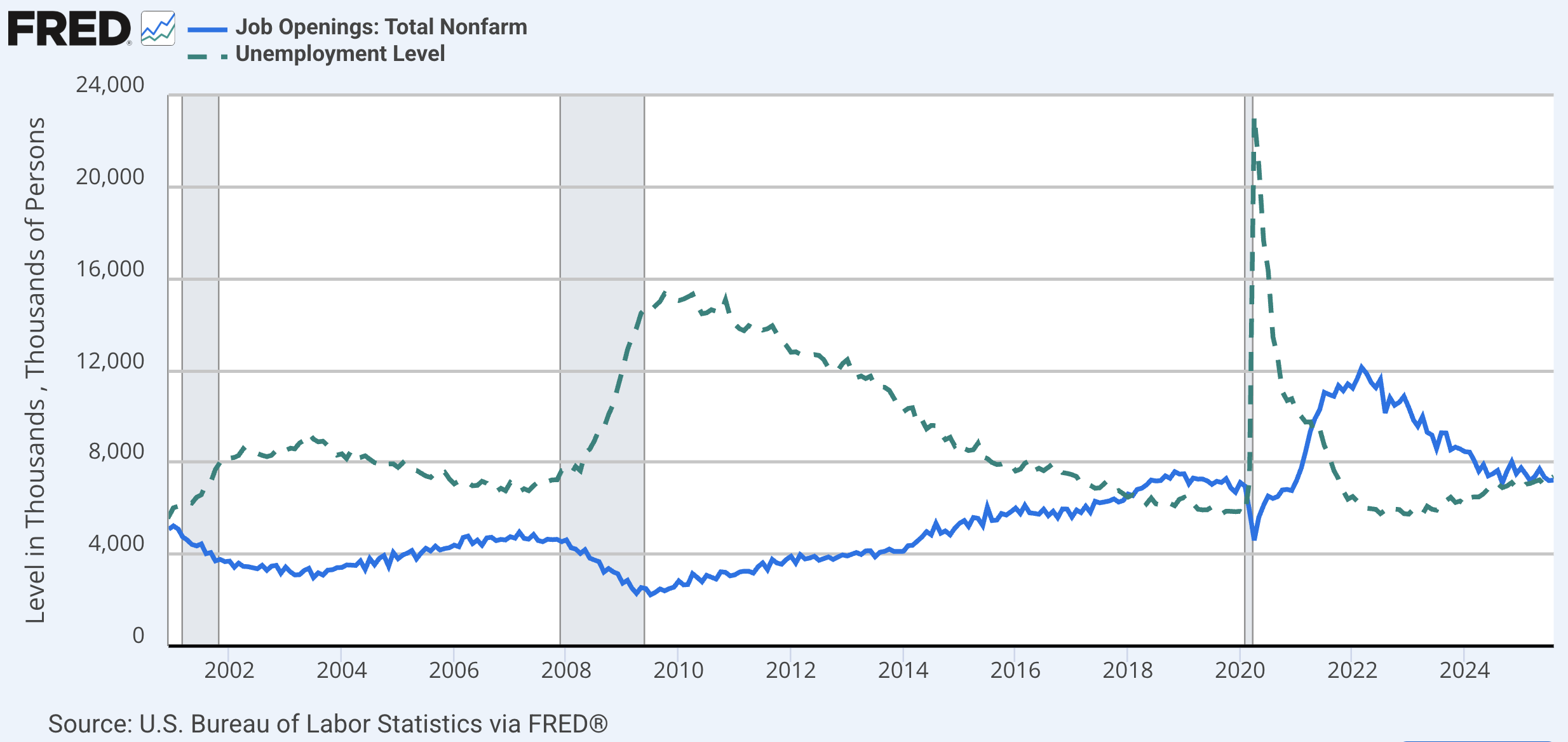
Before a recession, unemployment is lowest and job openings are highest, which means workers have the most bargaining power.
Immediately after a recession, the number of unemployed workers searching for work is highest while job openings is lowest, which means workers have very little bargaining power.
Thus, worker bargaining power varies over the business cycle and is negatively related to the unemployment rate.
Source
# Libraries
from fredapi import Fred
import pandas as pd
# Read data
fred_api_key = pd.read_csv('fred_api_key.txt', header=None).iloc[0,0]
fred = Fred(api_key=fred_api_key)
data = fred.get_series('JTSJOL').to_frame(name='Vacancies')
# append unemployment rate to data
data['Unemployment Rate'] = fred.get_series('UNRATE')
# append labor force to data
data['Labor Force'] = fred.get_series('CLF16OV')
# create series for job vacancy rate
data['Job Vacancy Rate'] = 100*data['Vacancies'] / data['Labor Force']
# create scatter plot of data unemployment vs vacancies
import matplotlib.pyplot as plt
# create list of subsamples of data for 2000 to 2010, 2010 to 2020, and 2020 to 2024
subsamples = [
    data['2000-01-01':'2009-12-31'],
    data['2010-01-01':'2019-12-31'],
    data['2022-01-01':'2025-12-31']
]
subsamples_legends = ['2000-2009', '2010-2019', '2022-2025']
# plot each subsample in different color
colors = ['red', 'green', 'blue']
for i, subsample in enumerate(subsamples):
    plt.scatter(subsample['Unemployment Rate'], subsample['Job Vacancy Rate'], color=colors[i], label=subsamples_legends[i])
plt.legend()
plt.xlabel('Unemployment Rate (%)')
plt.ylabel('Job Vacancy Rate (%)')
plt.title('Beveridge Curves')
# add grid
plt.grid()
# change figure size to 6.5 by 4.5 inches
plt.gcf().set_size_inches(8.5, 4)
plt.show()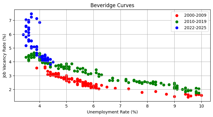
Job openings as a share of the labor force is known as the job vacancy rate.
Possible reasons for the BC shifting out: 1) lower matching efficiency or longer search times, 2) decreased turnover/churn in labor market, 3) sectoral/structural mismatch, 4) firms preferring to hire previously employed vs unemployed workers
Nominal Wage
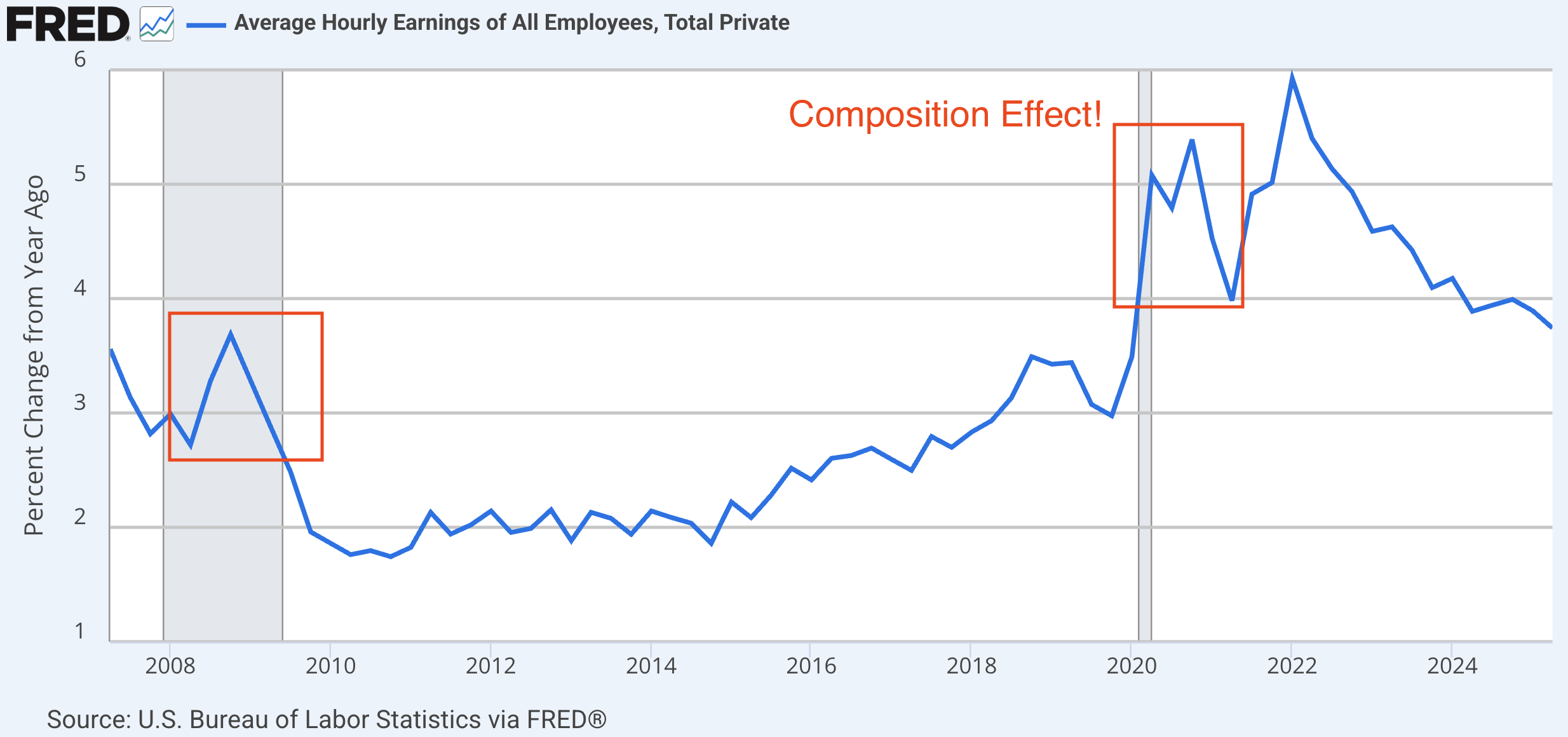
This series includes salaried workers but earnings do not include benefits.
Nominal wage growth fell after Great Recession and increased in expansion.
This series suffers from a composition effect, e.g., during COVID lower-income workers were more likely to become unemployed which drives up the average hourly rate in 2020 and 2021.
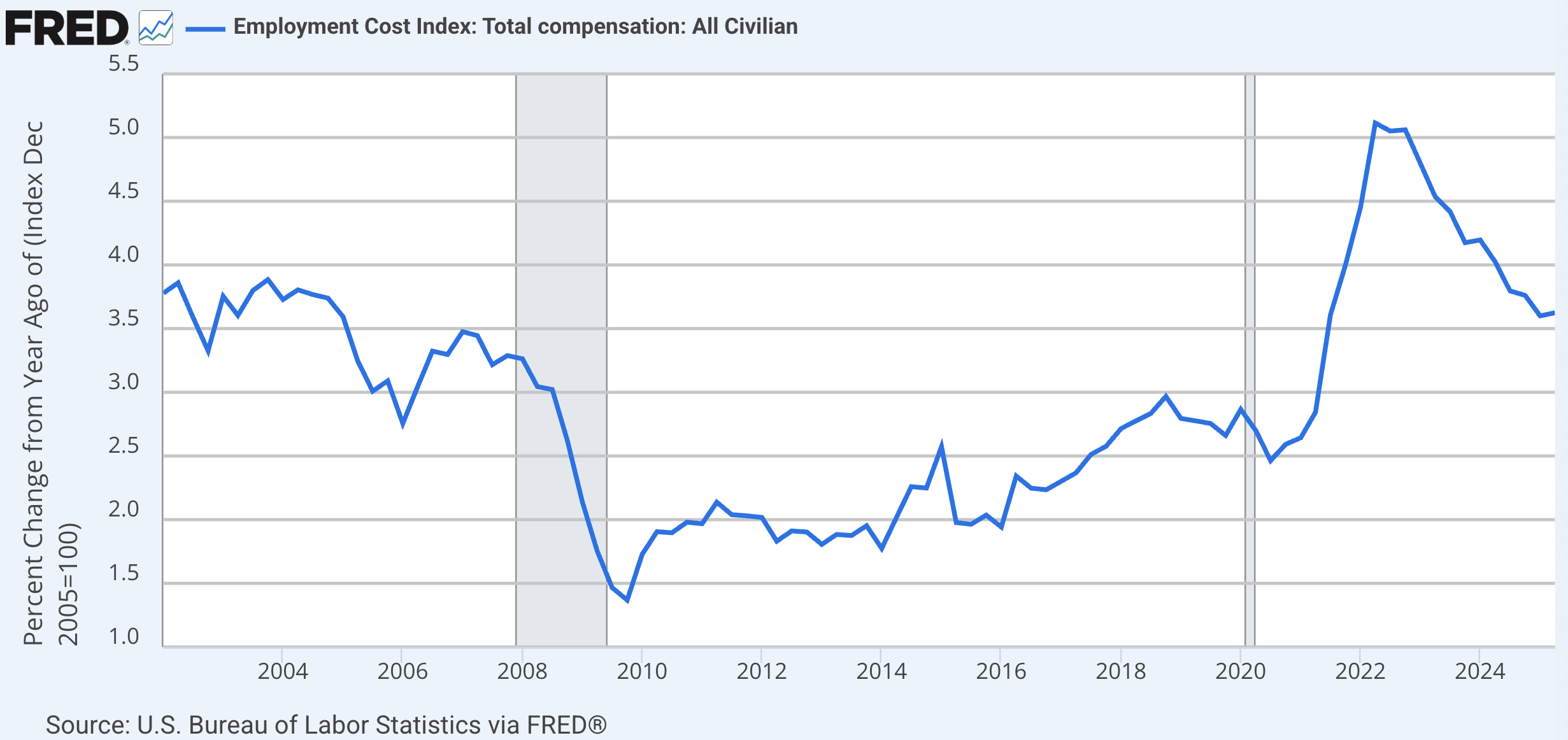
Employment Cost Index (ECI) is a fixed-weight index of nominal employer hourly wage costs (excluding benefits) across a constant “basket” of occupations.
Thus, it is not affected by composition changes.
The growth rate of the nominal wage is clearly procyclical, i.e., it falls in recessions and rises in expansions.
Source
# Libraries
from fredapi import Fred
import pandas as pd
# Read data
fred_api_key = pd.read_csv('fred_api_key.txt', header=None).iloc[0,0]
fred = Fred(api_key=fred_api_key)
# get series for ECI (ECIALLCIV index)
data = fred.get_series('ECIALLCIV').to_frame(name='ECI')
# append unemployment rate to data
data['Unemployment Rate'] = fred.get_series('UNRATE')
# resample date to a quarterly frequency use the end of period value
data = data.resample('QE').last()
# append ECI year-over-year growth rate to data
data['ECI Growth Rate'] = 400*data['ECI'].pct_change()
# create scatter plot of data ECI growth vs unemployment rate
import matplotlib.pyplot as plt
# create list of subsamples of data for 2000 to 2010, 2010 to 2020, and 2020 to 2024
subsamples = [
    data['2001-06-01':'2009-12-31'],
    data['2010-01-01':'2019-12-31'],
    data['2020-01-01':'2025-08-31']
]
subsamples_legends = ['2000-2009', '2010-2019', '2020-2025']
# plot each subsample in different color
colors = ['red', 'green', 'blue']
for i, subsample in enumerate(subsamples):
    plt.scatter(subsample['Unemployment Rate'], subsample['ECI Growth Rate'], color=colors[i], label=subsamples_legends[i])
plt.legend()
plt.xlabel('Unemployment Rate (%)')
plt.ylabel('ECI Growth Rate (%)')
# add grid
plt.grid()
# change figure size to 6.5 by 4.5 inches
plt.gcf().set_size_inches(8.5, 4)

# add best fit curve to scatter plot
import numpy as np
# import linear regression from statsmodels
import statsmodels.api as sm
# fit linear regression model to each subsample and plot best fit line
for i, subsample in enumerate(subsamples):
    ur = subsample['Unemployment Rate']
    # create regressors with ur, constant
    X = pd.DataFrame({
        'const': 1,
        'ur': ur,
    })
    y = subsample['ECI Growth Rate']
    model = sm.OLS(y, X).fit()
    x_fit = np.linspace(X['ur'].min(), X['ur'].max(), 100)
    y_fit = model.predict(pd.DataFrame({  'const': 1, 'ur': x_fit}))
    plt.plot(x_fit, y_fit, color=colors[i], linestyle='--')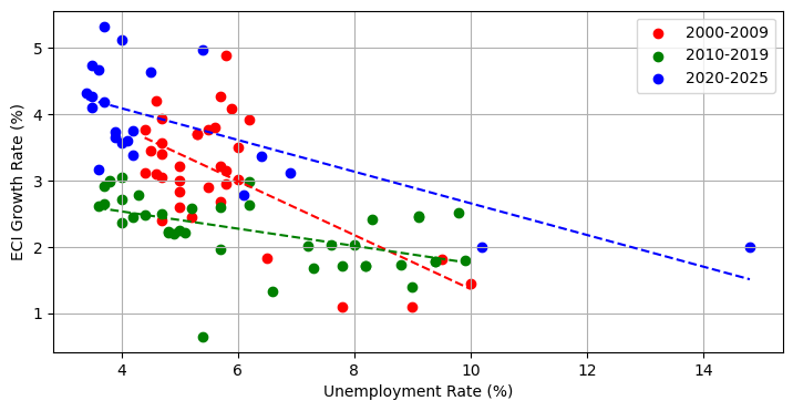
ECI, i.e., the nominal wage, is negatively correlated with unemployment rate.
From AP/Intro Macro, this looks like an empirical version of the Phillips Curve, which we’ll develop the theory for.
Wage and Price Determination
Wage setting is given by
is the nominal wage rate
is the expected price level
if workers expect the price level to increase by
they will (eventually) demand an increase in
is the unemployment rate
In a recession, when is high, worker bargaining power (BP) is low,
workers are willing to accept lower
are all other things that affect worker bargaining power, e.g.,
minimum wage
unemployment insurance benefits
laws that affect the collective bargaining power (of unions)
employment protections
foreign labor supply or automation
If something besides leads to higher worker BP, then
it represented by
worker can demand higher
Production Function
A Cobb-Douglas constant-returns-to-scale (CRS) production function is .
The factors of production are the capital stock () and labor ().
is labor productivity, and is the elasticity of output to changes in the capital stock.
The production function determines a firm’s cost function, e.g., factor prices are equal to their marginal products when markets are perfectly competitive, which you learn in intermediate microeconomic theory.
For the labor market, we care about labor as an input and capital accumulation is more likely to be important for long-run growth than it is in the short to medium-run.
Let’s assume:
Constant productivity, .
Zero output elasticity of capital,
Thus our short to medium-run production function is , i.e., if is employment then each worker produces one thing.
Price Setting
If is the only factor of production, then is the only factor price (i.e., marginal cost) paid by the firm.
If the average firm competes in a monopolistic product market, then they have pricing power and receive positive profits in equilibrium.
Denote a firm’s profit margin (or markup) by the parameter .
Thus, price setting is given by , i.e., firms set price at a markup above marginal cost.
Wage-Price Spiral
After the COVID shutdowns and the expansionary monetary and fiscal policy responses, there was a lot of inflation relative to the 20 years before COVID.
In the labor market model, that is a situation where , i.e., the actual price is higher than what worker’s expected.
Wage setting: Workers then begin to expect higher prices, , which eventually leads to them demanding higher wages to maintain the buying power of their income.
Price setting: Firms eventually pass the higher costs onto their customers,
But when workers see prices rise again, they and the loop repeats, which is the wage-price spiral.
This is the theory behind a major debate about whether inflation following COVID would be transitory or permanent.
Labor Market Model
The labor market model consists of wage and price setting equations
For equilibrium to exist, , otherwise wages and prices are moving around (disequilibrium).
Thus, we can rewrite both equations in terms of the actual real wage rate
Unemployment
In AP/intro macro, we learn that unemployment is either frictional, structural, cyclical or seasonal.
The labor market is a medium-run model (with a 2-5 year horizon), so we can ignore seasonal unemployment.
In a medium-run equilibrium, that natural unemployment rate () consists of frictional and structural unemployment.
In the short-run, the unemployment rate fluctuates cyclically and can be less than or greater than the natural unemployment rate, e.g., the short-run unenmployment rate is above in a recession.
Medium-run Equilibrium
The labor market in equilibrium determines the natural, or medium-run, unemployment rate, .
The short-run unemployment rate is moving toward in the medium-run.
In a graph of the labor market, is at the intersection of WS and PS.
Source
m = 0.1
import matplotlib.pyplot as plt
import numpy as np

x = np.linspace(0, 9, 100)
# plot a flat line at 1/(1+m) and label it PS
plt.plot(x, 1/(1+m)*np.ones_like(x), color='r', linestyle='-')
plt.text(8.5, 1, 'PS', horizontalalignment='right')
# plot a downward sloping line and label it WS
y = (1.75 - 0.15*x) / (1 + m)
plt.plot(x, y, color='b', linestyle='-')
plt.text(8.5, y[-1], 'WS', horizontalalignment='right')
# add a vertical dashed line at x=5 from y = 0 to y = 0.9 and label it u_n
plt.plot([5, 5], [0, 0.9], color='black', linewidth=0.5, ls='--')
plt.text(5, -.1, '$u_n$', verticalalignment='bottom', horizontalalignment='center')
# set ylims to 0 to 2
plt.ylim(0, 2/(1+m))
# remove tick labels
plt.xticks([])
plt.yticks([])
# label the vertical axis W/P at the top
plt.ylabel(r'$\frac{W}{P}$', rotation=0, loc = 'top')
# label the horizontal axis u at the right
plt.xlabel(r'$u$', rotation=0, loc = 'right')
# remove the box side on top and right
plt.gca().spines['top'].set_visible(False)
plt.gca().spines['right'].set_visible(False)
# change figure size to 5 by 6 inches
plt.gcf().set_size_inches(5, 4)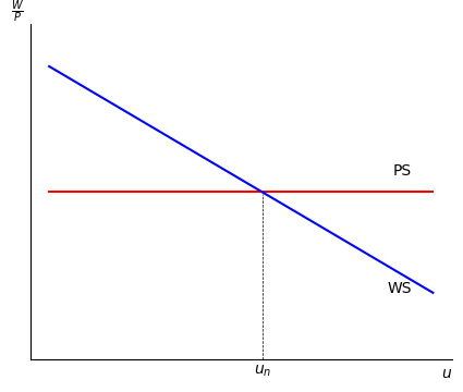
Source
m = 0.1
import matplotlib.pyplot as plt
import numpy as np

x = np.linspace(0, 9, 100)
# plot a flat line at 1/(1+m) and label it PS
plt.plot(x, 1/(1+m)*np.ones_like(x), color='r', linestyle='-')
plt.text(8.5, 1, 'PS', horizontalalignment='right')
# plot a downward sloping line and label it WS
y = (1.5 - 0.15*x) / (1 + m)
plt.plot(x, y, color='b', linestyle='-')
plt.text(8.5, y[-1], 'WS', horizontalalignment='right')
# add a vertical dashed line at x=5 from y = 0 to y = 0.9 and label it u_n
plt.plot([3.3, 3.3], [0, 0.9], color='black', linewidth=0.5, ls='--')
plt.text(3.3, -.1, '$u_n$', verticalalignment='bottom', horizontalalignment='center')
# set ylims to 0 to 2
plt.ylim(0, 1.5)
# remove tick labels
plt.xticks([])
plt.yticks([])
# label the vertical axis W/P at the top
plt.ylabel(r'$\frac{W}{P}$', rotation=0, loc = 'top')
# label the horizontal axis u at the right
plt.xlabel(r'$u$', rotation=0, loc = 'right')
# remove the box side on top and right
plt.gca().spines['top'].set_visible(False)
plt.gca().spines['right'].set_visible(False)
# change figure size to 5 by 6 inches
plt.gcf().set_size_inches(5, 4)
# add dashed vertical line at x = 5
plt.plot([6, 6], [0, 0.9], color='black', linewidth=0.5, ls='--')
# add label at x = 6 for $u_{recession}$
plt.text(6, -.1, '$u_{recession}$', verticalalignment='bottom', horizontalalignment='center');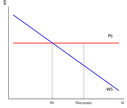
In a recession, is above , and is cyclical unemployment.
At , the real wage offered by firms exceeds the real wage firms are willing to accept.
Thus firms increase hiring and unemployed workers transition to employment.
As the unemployment rate falls, workers can demand higher real wages.
After a few years, the real wage firms offer equals the real wages workers want at .
Experiment
Source
m = 0.1
import matplotlib.pyplot as plt
import numpy as np

x = np.linspace(0, 9, 100)
# plot a flat line at 1/(1+m) and label it PS
plt.plot(x, 1/(1+m)*np.ones_like(x), color='r', linestyle='-')
plt.text(8, 1, 'PS', horizontalalignment='right')
# plot a downward sloping line and label it WS
y = (1.5 - 0.15*x) / (1 + m)
plt.plot(x, y, color='r', linestyle='-')
plt.text(8.5, y[-1], 'WS', horizontalalignment='right')
plt.plot(x, y+0.36, color='b', linestyle='-')
plt.text(8.5, y[-1]+0.36, 'WS\'', horizontalalignment='right')
# add a vertical dashed line at x=5 from y = 0 to y = 0.9 and label it u_n
plt.plot([3.3, 3.3], [0, 1.27], color='black', linewidth=0.5, ls='--')
plt.text(3.3, -.1, '$u_n$', verticalalignment='bottom', horizontalalignment='center')
# set ylims to 0 to 2
plt.ylim(0, 1.5)
# remove tick labels
plt.xticks([])
plt.yticks([])
# label the vertical axis W/P at the top
plt.ylabel(r'$\frac{W}{P}$', rotation=0, loc = 'top')
# label the horizontal axis u at the right
plt.xlabel(r'$u$', rotation=0, loc = 'right')
# remove the box side on top and right
plt.gca().spines['top'].set_visible(False)
plt.gca().spines['right'].set_visible(False)
# change figure size to 5 by 6 inches
plt.gcf().set_size_inches(5, 4)
# add dashed vertical line at x = 5
plt.plot([6, 6], [0, 0.9], color='black', linewidth=0.5, ls='--')
# add label at x = 6 for $u_{recession}$
plt.text(6, -.1, '$u_n\'$', verticalalignment='bottom', horizontalalignment='center')
# add up arrow between two WS curves
plt.annotate('', xy=(7, .75), xytext=(7, .42),
             arrowprops=dict(arrowstyle='->'));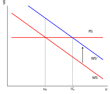
Suppose a policy increases worker bargaining power, .
Workers demand higher real wages reflected by an increase in WS.
At , real wages demand exceed real wages offered, so workers quit to search for higher paying work, or firms layoff workers because they cannot afford to pay them.
Employed workers transition to unemployment and the short-run unemployment rate increases to the new natural unemployment rate where there is more frictional unemployment in equilibrium than before.