Growth Model - Intermediate Macro

by Professor Throckmorton
for Intermediate Macro
W&M ECON 304
Slides

Stock vs Flow Variables¶

A stock variable is measured at a specific point in time. It represents a quantity that exists at that instant (i.e., a snapshot or balance).
A flow variable is measured over an interval of time. It represents a rate of change or movement over time.

Stock	Inflow	Outflow
Lake	Rain	Evaporation
National debt	Budget deficit	Budget surplus
Wealth	Income	Consumption
Capital	Investment	Depreciation

Capital Accumulation¶

	Start of 2025	Flow	End of 2025
Old Capital	$K_{2025}$	Depreciation	$(1-\delta)K_{2025}$
New Capital	0	Investment	+ $I_{2025}$
Capital Stock			$= K_{2026}$

$K_{2026} = (1-\delta)K_{2025} + I_{2025}$
Capital stock available for production in 2026 is the sum of
- the non-depreciated old capital at the start of 2025
- and investment in new capital over the course of 2025.

Capital Law of Motion

The above accounting of the capital stock should apply in any year

K_{t+1} = (1-\delta)K_{t} + I_{t}

(1)

Which can be expressed as a difference equation to track the changes in the capital stock

\Delta K_{t+1} = K_{t+1} - K_t = I_{t} - \delta K_{t}

(2)

If $I_{t} = \delta K_{t}$ , then the capital stock is “steady” and the growth model is in an equilibrium.
Assuming a constant number of workers, this can be written as

\frac{\Delta K_{t+1}}{N} = \frac{I_{t}}{N}- \delta \frac{K_{t}}{N}

(3)

Savings¶

What is $I_t$ ?
Suppose households either consumer or save their income

Y_t = C_t + S_t

(4)

Assume that households save a fixed fraction of their income. Let the savings function be $S_t = sY_t$ , where $s$ is the savings rate.
Assume that there is a financial market equilibrium where $S_t = I_t$ .
All excess wealth from households, $S_t$ , gets converted by banks into loans, bonds, or stocks, which are then used to invest in new capital, $I_t$ .
Thus, $I_t = sY_t$ .

Solow Growth Model¶

This Solow Growth Model has 3 variables $\{Y,K,I\}$ (with $N$ fixed) in the following 3 equations

\begin{gather*} \frac{Y_t}{N} = \left(\frac{K_t}{N}\right)^\alpha \\ \frac{\Delta K_{t+1}}{N} = \frac{I_{t}}{N} - \delta \frac{K_{t}}{N} \\ \frac{I_t}{N} = s\frac{Y_t}{N} \end{gather*}

(5)

There are also 3 parameters
1. The output elasticity of capital, $\alpha$ .
2. The depreciation rate, $\delta$ .
3. The savings rate, $s$ .
We could add a 4th variable for consumption, $C$ , and equation
$Y = C + I$
(6)
which looks like the expenditure approach to GDP without the $G$ and $NX$ .

import numpy as np
import matplotlib.pyplot as plt

alpha = 0.4
s = 0.5
delta = 0.1
k = np.linspace(0, 30, 200)
y = k ** alpha
i = s*y
dep = delta*k

# Plot
fig, ax = plt.subplots(figsize=(6, 3))
# Curves
ax.plot(k, y, label=r"$Y_t/N = (K_t/N)^\alpha$", color="blue")
ax.plot(k, i, label=r"$I_t/N = s Y_t/N$", linestyle="--", color="green")
ax.plot(k, dep, label=r"$\delta K_t/N$", linestyle="--", color="red")
ax.legend(loc="lower right")
# Vertical lines
ax.axvline(x=15, color="black", linestyle=":")
# Horizontal lines
ax.axhline(y=3, color="black", linestyle=":")
ax.axhline(y=1.5, color="black", linestyle=":")
# Labels
ax.text(15, -0.4, r"$\frac{K^*}{N}$", fontsize=12, ha='center')
ax.text(-1, 2.9, r"$\frac{Y^*}{N}$", fontsize=12, ha='center',color="blue")
ax.text(-1, 1.4, r"$\frac{I^*}{N}$", fontsize=12, ha='center',color="green")
ax.set_xlabel("$K/N$", loc="right")
ax.set_ylabel("$Y/N$", loc="top")
# Styling
ax.grid(); ax.autoscale(tight=True);
# remove ticks
ax.set_xticks([]); ax.set_yticks([]);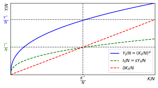

The solid-blue line is the production function.
The dashed-green line is the investment/savings function.
The dashed-red line is the depreciation function.
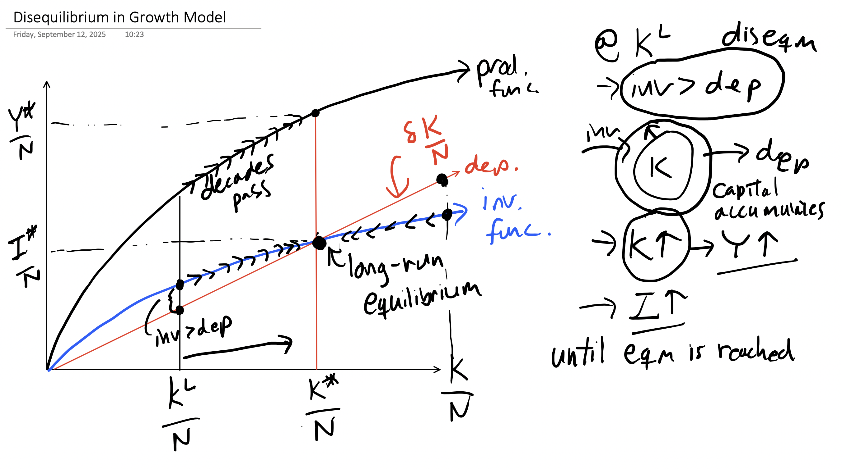
If investment equal depreciation, then capital is at its long-run equilibrium or steady-state level.

Steady State¶

Another name for a long-run equilibrium in a dynamic economic model is steady state.
In this model, the capital stock is a state variable because given its value in any year allows us to determine the level of output, investment, and consumption per person.
Thus, if we assume capital is at its steady state, then we can calculate the steady-state, or long-run equilibrium, values for the other variables in the model.

If the model starts in steady state, then it stays there until something happens. Until then $K_{t+1} = K_t = K^*$ or $\Delta K_{t+1} = 0$ .
The steady-state system of equations is
$\begin{gather*} \frac{Y^*}{N} = \left(\frac{K^*}{N}\right)^\alpha \\ 0 = \frac{I^*}{N} - \delta \frac{K^*}{N} \\ \frac{I^*}{N} = s\frac{Y^*}{N} \end{gather*}$
(7)
Combining the steady-state equations yields
$\begin{gather*} s\left(\frac{K^*}{N}\right)^\alpha = \delta \frac{K^*}{N} \end{gather*}$
(8)
The solution for steady-state capital per worker is
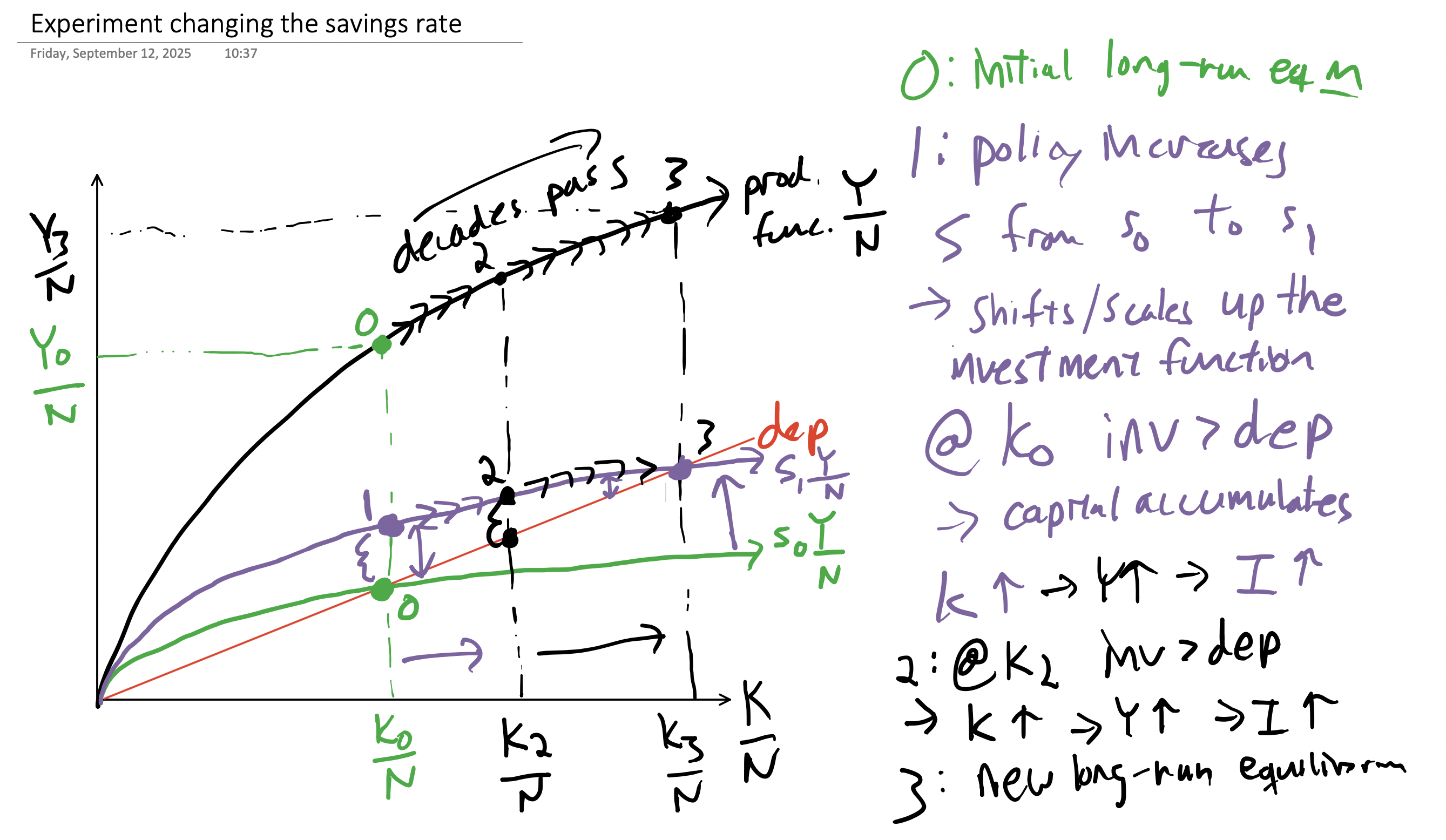
$\begin{gather*} \frac{K^*}{N} = \left(\frac{s}{\delta}\right)^{\frac{1}{1-\alpha}} \end{gather*}$
(9)

Equilibrium¶

Savings¶

Technological Progress¶

We can relax the assumptions
- that $A = 1$ by assuming $A$ grows at rate $g_A$ .
- that $N$ is fixed by assuming $N$ grows at rate $g_N$ .
However, $A$ increasing over time complicates our illustration of the model since output per worker would always be increasing.
We need to write production in terms of output per effective worker
$\left(\frac{Y}{AN}\right)_t = \left(\frac{K}{AN}\right)^\alpha_t$
(10)

Equilibrium

Now the relevant state of the model is how much capital is available to each effective worker, $K/(AN)$ at any time $t$ .
Investment is still an inflow and depreciation is still an outflow to the capital stock, as before.
But now there are two new outflows, $g_A$ and $g_N$ , because $A$ and $N$ appear in the denominator of the state.
The equilibrium (steady-state) condition is still that inflow equals outflow
$\left(\frac{I}{AN}\right)^* = (\delta + g_A + g_N) \left(\frac{K}{AN}\right)^*$
(11)
Dynamically, the capital (per effective worker) accumulation equation becomes
$\Delta \left(\frac{K}{AN}\right)_{t+1} = \left(\frac{I}{AN}\right)_t - (\delta + g_A + g_N) \left(\frac{K}{AN}\right)_t$
(12)

Balanced Growth

The following table is based on Blanchard, Macroeconomics (9th Edition, 2025), Chapter 12, Page 247, Table 12-1

Variable	Growth Rate
$\frac{K}{AN}, \frac{Y}{AN}$	0
$\frac{K}{N}, \frac{Y}{N}$	$g_A$
$K, Y, AN$	$g_A + g_N$

“Because output, capital, and effective labor all grow at the same rate in steady state, the steady state of this economy is also called a state of balanced growth.”
“Changes in the saving rate do not affect the steady-state growth rate. But changes in the saving rate do increase the steady-state level of output per effective worker.” (i.e., the same result as the model with $A=1$ and $N$ fixed)