Financial Markets

by Professor Throckmorton
for Intermediate Macro
W&M ECON 304
Slides

Summary¶

• Define present value and arbitrage

• Arbitrage $\rightarrow$ equal expected returns, i.e., a financial market equilibrium

• Define Yield-to-maturity and interpret the yield curve

• Derive relationship between interest rates and stock prices

Present Value¶

• Present value is the current worth of a future payment or stream of payments, discounted back using an appropriate interest rate to reflect the time value of money.

• Applying present value allows us to price any asset, e.g., bond, stock, mortgage

• Since present value depends on market expectations, current asset prices have information about expectations

• Asset pays principal plus (expected) interest, compounding over time

• Present value of $\$1$ received next year is discounted by $1+i_t$

• Present value of $\$1$ received in 2 years is discounted by $(1+i_t)(1+i_{t+1}^e)$

• What’s important is to discount future cash flow according to when it’s received.

• Recall a simple loan/one-period zero-coupon discount bond (e.g., T-Bill)

  $$\begin{gather*} P_B = \frac{\textrm{Face Value}}{1+i} \end{gather*}$$

  (1)

• Current market price equals face value (future cash-flow) discounted to present by interest rate

• $P_B$ is initial investment/loan given by market price, Face Value is known, this implies an interest rate, $i$ (a.k.a. yield to maturity)

Arbitrage¶

• General use: buy thing at low price in one market and sell it at a higher price in a different market

• For example, you could buy laptops for cash on college campuses and then list them on ebay at a higher price.

• In finance, arbitrage refers to buying/selling assets depending on relative expected returns

• For example, sell an asset with a high price/low expected return, then buy a different asset with low price/high expected return.

• Goal: maximize expected return on a portfolio of assets

Portfolio Choice¶

• Properties of bonds

  • Credit/default risk: who issued them and what’s the risk premium/spread?

  • Maturity: how long until bond pays face value?

  • Discount/Coupons: does bond also pay coupons?

• Consider a small portfolio

  • Credit/default risk: bonds issued by U.S. government, so no default/credit risk

  • Maturity: either 1 or 2 years

    • 1-year bond has price $P_{1,t}$ and pays $F.V.$ in 1 year

    • 2-year bond has price $P_{2,t}$ and pays $F.V.$ in 2 years

  • Discount/Coupons: discount bonds only, no coupons, e.g., Treasury bills

• 2-year bond is transferable and could be sold after 1 year

  • Q: What is price of 2-year bond with 1-year left?

  • A: The price of a 1-year bond at that time.

• Q: How do we manage this portfolio?

• To compare cashflow next year, sell the 2-year bond next year at expected 1-year bond price, $P^e_{1,t+1}$.

• Divide by bond price to “invest” $\$1$ in each choice.

• The return on $\$1$ worth of a 1-year bond is $F.V./P_{1,t}$ vs. the expected return on $\$1$ worth of a 2-year bond, which is $P^e_{1,t+1}/P_{2,t}$

• Goal: maximize expected return on portfolio

  • 1-year bond return: $F.V./P_{1,t}$

  • 2-year bond expected return: $P_{1,t+1}^e/P_{2,t}$

• Three possible cases:

  1. Disequilibrium (arbitrage opportunity):
     $F.V./P_{1,t} < P_{1,t+1}^e/P_{2,t}$
     $\rightarrow$ sell 1-year ($\downarrow P_{1,t}$) and buy 2-year ($\uparrow P_{2,t}$)
     $\rightarrow$ expected returns equalize

  2. Disequilibrium (arbitrage opportunity):
     $F.V./P_{1,t} > P_{1,t+1}^e/P_{2,t}$
     $\rightarrow$ buy 1-year ($\uparrow P_{1,t}$) and sell 2-year ($\downarrow P_{2,t}$)
     $\rightarrow$ expected returns equalize

  3. Equilibrium: $F.V./P_{1,t} = P_{1,t+1}^e/P_{2,t}$ (equal returns)
     $\rightarrow$ no incentive to rebalance portfolios

• Cases 1) and 2) are arbitrage opportunities that lead to the equilibrium where there is no more arbitrage.

Equilibrium 2-year Bond Price¶

• In equilibrium, 1-year return $=$ expected 2-yr return

• Recall present value formula for 1-year bond price

• Combine those

• Update 1-year bond price forward one year, take expectation

• Substitute that into 2-year bond price

• This is the present value (i.e., asset pricing) formula for a 2-year discount bond.

Yield to Maturity/Curve¶

• Yield to Maturity (YtM): the annual interest rate a bond holder receives if bond is held to maturity

• I.e., YtM is the constant interest rate that equates current bond price with present value of all future cash-flow, e.g., for an $N$-year discount bond,

  $$\begin{gather*} P_{N,t} = \frac{F.V.}{(1+i_{N,t})^N} \end{gather*}$$

  (7)

  where $i_{N,t}$ is $N$-year YtM

• We know $P$ and cash flow, so we can calculate all YtM

• Yield Curve: a graph/table of YtM as function of maturity for bonds that have same credit/default risk, e.g., U.S. Treasuries

• Combine bond market equilibrium with YtM definition

  $$\begin{gather*} P_{2,t} = \frac{F.V.}{(1+i_{1,t})(1+i_{1,t+1}^e)} = \frac{F.V.}{(1+i_{2,t})^2} \end{gather*}$$

  (8)

• Since numerators are equal, then denominators are equal

  $$\begin{gather*} (1+i_{1,t})(1+i_{1,t+1}^e) =(1+i_{2,t})^2 \end{gather*}$$

  (9)

• Equation is nonlinear, so let’s linearize it! Recall

  $$\begin{gather*} \log((1+x)(1+y)) = \log(1+x) + \log(1+y) \log(1+x) \approx x \textrm{ if $x$ is small} \log((1+y)^b) = b \log (1+y) \end{gather*}$$

  (10)

  where $\log$ is the natural logarithm

• Take logs and use properties

  $$\begin{gather*} (1+i_{1,t})(1+i_{1,t+1}^e) =(1+i_{2,t})^2 \rightarrow \log(1+i_{1,t}) + \log(1+i_{1,t+1}^e) = \log((1+i_{2,t})^2) \rightarrow \log(1+i_{1,t}) + \log(1+i_{1,t+1}^e) = 2 \log(1+i_{2,t}) \rightarrow i_{1,t} + i_{1,t+1}^e = 2 i_{2,t} \end{gather*}$$

  (11)

• 2-year YtM is average of 1-year rates

  $$\begin{gather*} i_{2,t} = (i_{1,t} + i_{1,t+1}^e)/2 \end{gather*}$$

  (12)

• Expected 1-year rate (predicted)

  $$\begin{gather*} i_{1,t+1}^e = 2i_{2,t} - i_{1,t} \end{gather*}$$

  (13)

Expectations Hypothesis¶

• Expectations hypothesis: the long-term rate is determined purely by current and future expected short-term rates

• Since we can calculate YtM from current bond prices, the expectations hypothesis leads to a prediction about expected future short-term rates

• E.g, if $i_{2,t}$ falls, then $i_{1,t+1}^e$ also falls

• Q: When would $i_{1,t+1}$ actually decrease?
  A: When the central bank sets a lower rate (in a recession).

Expectations hypothesis gives three cases for interpreting yield curve

• Upward sloping: $i_{2,t} > i_{1,t}$
  $\rightarrow$ $i_{1,t+1}^e > i_{1,t}$, i.e., central bank expected to raise rate
  $\rightarrow$ bond market expects boom/expansion

• Downward sloping ({\color{red} i.e., inverted}): $i_{2,t} < i_{1,t}$
  $\rightarrow$ $i_{1,t+1}^e < i_{1,t}$, i.e., central bank expected to lower rate
  $\rightarrow$ bond market expects bust/recession

• Flat (typically before recessions): $i_{2,t} = i_{1,t}$
  $\rightarrow$ $i_{1,t+1}^e = i_{1,t}$
  $\rightarrow$ bond market expecting move from boom to bust

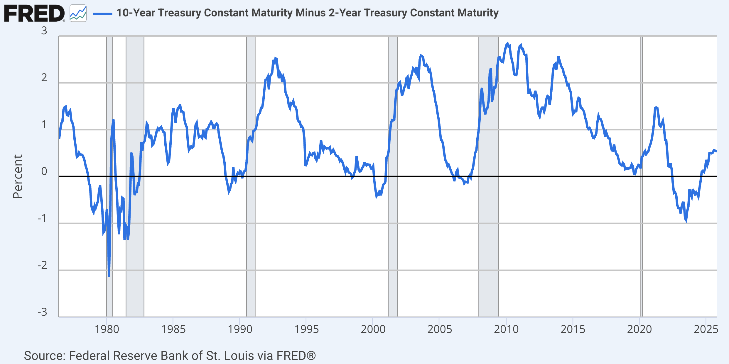
It’s usually upward sloping, but downward sloping ($i_{10,t} - i_{2,t} < 0$)before recessions?
10-Year Treasury Constant Maturity Minus 2-Year Treasury Constant Maturity (T10Y2Y)

Stock Market¶

• Bonds and stocks both store wealth (i.e., they are substitutable)

• New goal: maximize expected return on portfolio of 1-yr bond and a stock

• Stock characteristics
  - $Q_t$ is current price
  - $D_{t+1}^e$ is expected dividend (e.g., random, could be zero)
  - $Q_{t+1}^e$ is expected future price

• Q: What’s the cash flow on a stock if you sell it after a year?
  A: The expected dividend plus the expected sale price.

Portfolio Choice Problem

Normalize

• Time horizon $= 1$ year

• Initial investment $= \$1$

• $x$ is the risk premium, i.e., the additional return the portfolio manager wants to compensate them for the price risk of holding a stock

Goal: Maximize expected portfolio return

1. Disequilibrium (arbitrage opportunity):
   1-yr bond return $<$ expected stock return
   $\rightarrow$ sell 1-yr bond ($\downarrow P_{1,t}$) and buy stock ($\uparrow Q_t$)
   $\rightarrow$ expected returns equalize

2. Disequilibrium (arbitrage opportunity):
   1-yr bond return $>$ expected stock return
   $\rightarrow$ buy 1-yr bond ($\uparrow P_{1,t}$) and sell stock ($\downarrow Q_t$)
   $\rightarrow$ expected returns equalize

3. Equilibrium: 1-yr bond return $=$ expected stock return
   $\rightarrow$ no incentive to reallocate portfolio
   (equal expected returns / no more arbitrage opportunties)

Stock Price¶

• Assume equilibrium and solve for $Q_t$ (with risk premium)

  $$\begin{gather*} Q_t = \frac{D_{t+1}^e + Q_{t+1}^e}{1+i_{1,t}+ x} \end{gather*}$$

  (15)

• Update one period and take expectation

  $$\begin{gather*} Q_{t+1}^e = \frac{D_{t+2}^e + Q_{t+2}^e}{1+i_{1,t+1}^e + x} \end{gather*}$$

  (16)

• Substitute 2 into 1

  $$\begin{gather*} Q_t = \frac{D_{t+1}^e}{1+i_{1,t}+ x} + \frac{D_{t+2}^e + Q_{t+2}^e}{(1+i_{1,t}+ x)(1+i_{1,t+1}^e + x)} \end{gather*}$$

  (17)

• This is a present value formula for a stock.

Fundamental Value

• Keep substituting out expected stock price

  $$\begin{gather*} Q_t = \frac{D_{t+1}^e}{1+i_{1,t}+ x} + \cdots + \frac{D_{t+N}^e + Q_{t+N}^e}{(1+i_{1,t}+ x)\times \cdots \times (1+i_{1,t+N-1}^e + x)} \end{gather*}$$

  (18)

• As $N \rightarrow \infty$, PV of expected stock price goes to zero

• Prediction: the fundamental value of a stock is just the present value of all future dividends (for a given risk premium)

Stock Price Summary

• Arbitrage $\rightarrow$ equal expected returns between a bond and stock (for a given risk premium)

• Stock price is positively related to expected dividends, i.e., expected future profitability

• Stock price is negatively related to (current or expected) short-term interest rates, e.g., news of higher future short-term interest rates lowers stock price

• If managers become more risk averse, then stock prices fall.

• The fundamental value of a stock is just the present value of all future dividends.