MA Model
by Professor Throckmorton
for Time Series Econometrics
W&M ECON 408
Slides
Wold Representation Theorem
Wold representation theorem: any covariance stationary series can be expressed as a linear combination of current and past white noise.
is a white noise process with mean 0 and variance .
, and , which ensures the process is stable.
, a.k.a. an innovation, represents new information that cannot be predicted using past values.
Key aspects
Generality: The Wold Representation is a general model that can represent any covariance stationary time series. This is why it is important for forecasting.
Linearity: The representation is a linear function of its innovations or “general linear process”.
Zero Mean: The theorem applies to zero-mean processes, but this is without loss of generality because any covariance stationary series can be expressed in deviations from its mean, .
Innovations: The Wold representation expresses a time series in terms of its current and past shocks/innovations.
Approximation: In practice, because an infinite distributed lag isn’t directly usable, models like moving average (MA), autoregressive (AR), and autoregressive moving average (ARMA) models are used to approximate the Wold representation.
MA Model
The moving average (MA) model expresses the current value of a series as a function of current and lagged unobservable shocks (or innovations)
The MA model of order , denoted as MA(), is defined as:
is the mean or intercept of the series.
is a white noise process with mean 0 and variance .
are the parameters of the model.
Key aspects
Stationarity: MA models are always stationary.
Approximation: Finite-order MA processes are a natural approximation to the Wold representation, which is MA().
Autocorrelation: The ACF of an MA() model cuts off after lag , i.e., the autocorrelations are zero beyond displacement . This is helpful in identifying a suitable MA model for time series data.
Forecasting: MA models are not forecastable more than steps ahead, apart from the unconditional mean, .
Invertibility: An MA model is invertible if it can be expressed as an autoregressive model with an infinite number of lags.
Unconditional Moments
The variance of an MA process depends on the order of the process and the variance of the white noise,
MA(1) Process:
MA() Process:
Autocorrelation Function
MA(1) Process:
for
, i.e., any series is perfectly correlated with itself
for
MA() process:
MA Model as DGP
Let’s compare a couple different MA models to their underlying white noise.
White noise:
MA(1):
MA(3):
# Import libraries
#   Plotting
import matplotlib.pyplot as plt
#   Scientific computing
import numpy as np
#   Data analysis
import pandas as pd
DIY simulation
# Assign parameters
T = 501; mu = 2; theta1 = 0.6; theta2 = 0.5; theta3 = 0.7;
# Draw random numbers
rng = np.random.default_rng(seed=0)
eps = rng.standard_normal(T)
# Simulate time series
y = np.zeros([T,3])
for t in range(3,T):
    y[t,0] = mu + eps[t]
    y[t,1] = mu + eps[t] + theta1*eps[t-1]
    y[t,2] = (mu + eps[t] + theta1*eps[t-1]
               + theta2*eps[t-2] + theta3*eps[t-3])
# Convert to DataFrame and plot
df = pd.DataFrame(y)
df.columns = ['White Noise','MA(1)','MA(3)']
df.plot(subplots=True,grid=True)array([<Axes: >, <Axes: >, <Axes: >], dtype=object)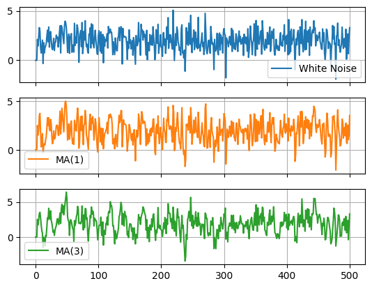
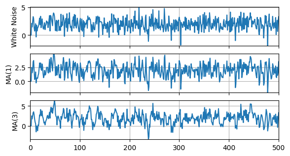
# Plot variables
fig, axs = plt.subplots(len(df.columns),figsize=(6.5,3.5))
for idx, ax in enumerate(axs.flat):
    col = df.columns[idx]
    y = df[col]
    ax.plot(y); ax.set_ylabel(col)
    ax.grid(); ax.autoscale(tight=True); ax.label_outer()
    print(f'{col}: \
E(y) = {y.mean():.2f}, \
Std(y) = {y.std():.2f}, \
AC(y) = {y.corr(y.shift(1)):.2f}')
White Noise: E(y) = 1.96, Std(y) = 1.03, AC(y) = -0.01
MA(1): E(y) = 1.95, Std(y) = 1.18, AC(y) = 0.43
MA(3): E(y) = 1.92, Std(y) = 1.43, AC(y) = 0.58
Using statsmodels
#   ARIMA Process
from statsmodels.tsa.arima_process import ArmaProcess as arma

# Set rng seed
rng = np.random.default_rng(seed=0)
# Create models (coefficients include zero lag)
wn = arma(ma=[1]);
ma1 = arma(ma=[1,theta1])
ma3 = arma(ma=[1,theta1,theta2,theta3])
# Simulate models
y = np.zeros([T,3])
y[:,0] = wn.generate_sample(T)
y[:,1] = ma1.generate_sample(T)
y[:,2] = ma3.generate_sample(T)
# Convert to DataFrame
df = pd.DataFrame(y)
df.columns = ['White Noise','MA(1)','MA(3)']
df.plot(subplots=True,grid=True)array([<Axes: >, <Axes: >, <Axes: >], dtype=object)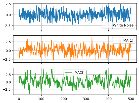
# Auto-correlation function
from statsmodels.graphics.tsaplots import plot_acf as acf
# Plot Autocorrelation Function
fig, ax = plt.subplots(figsize=(6.5,1.5))
acf(df['MA(3)'],ax)
ax.grid(); ax.autoscale(tight=True);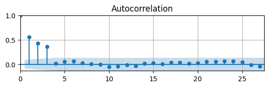
Since the DGDP is an MA(3), the ACF shows the correlations are only significant for the first 3 lags.
Estimating MA Model
In an MA model, the current value is expressed as a function of current and lagged unobservable shocks.
However, the error terms are not observed directly and must be inferred from the data and estimated parameters.
This creates a nonlinear relationship between the data and the model’s parameters.
The
statsmodelsmodule has a way to define an MA model and estimate its parameters.The general model is Autoregressive Integrated Moving Average Model, or ARIMA(), of which MA() is a special case.
The argument
order=(p,d,q)specifies the order for the autoregressive, integrated, and moving average components.See statsmodels for more information.
# ARIMA model
from statsmodels.tsa.arima.model import ARIMA
# Define model
mod = ARIMA(df['MA(3)'],order=(0,0,3))
# Estimate model
res = mod.fit()
summary = res.summary()
# Print summary tables
tab0 = summary.tables[0].as_html()
tab1 = summary.tables[1].as_html()
tab2 = summary.tables[2].as_html()
# print(tab0); print(tab1); print(tab2)| Dep. Variable: | MA(3) | No. Observations: | 501 |
|---|---|---|---|
| Model: | ARIMA(0, 0, 3) | Log Likelihood | -700.202 |
| Date: | Wed, 05 Feb 2025 | AIC | 1410.405 |
| Time: | 14:24:16 | BIC | 1431.488 |
| Sample: | 0-501 | HQIC | 1418.677 |
| coef | std err | z | P>|z| | [0.025 | 0.975] | |
|---|---|---|---|---|---|---|
| const | -0.1391 | 0.125 | -1.114 | 0.265 | -0.384 | 0.106 |
| ma.L1 | 0.6199 | 0.033 | 18.713 | 0.000 | 0.555 | 0.685 |
| ma.L2 | 0.5248 | 0.037 | 14.251 | 0.000 | 0.453 | 0.597 |
| ma.L3 | 0.6949 | 0.034 | 20.158 | 0.000 | 0.627 | 0.762 |
| sigma2 | 0.9540 | 0.064 | 14.819 | 0.000 | 0.828 | 1.080 |
| Ljung-Box (L1) (Q): | 0.09 | Jarque-Bera (JB): | 1.32 |
|---|---|---|---|
| Prob(Q): | 0.76 | Prob(JB): | 0.52 |
| Heteroskedasticity (H): | 1.08 | Skew: | 0.08 |
| Prob(H) (two-sided): | 0.61 | Kurtosis: | 2.80 |