ARIMA Model

by Professor Throckmorton
for Time Series Econometrics
W&M ECON 408
Slides

Summary¶

In a MA model, the current value is expressed as a function of current and lagged unobservable shocks.
In an AR model, the current value is expressed as a function of its lagged values plus an unobservable shock.
The general model is Autoregressive Integrated Moving Average Model, or ARIMA( $p,d,q$ ), of which MA are AR models are a special case.
$(p,d,q)$ specifies the order for the autoregressive, integrated, and moving average components, respectively.
Before we estimate ARIMA models, we should define the ARMA( $p,q$ ) model and the concept of integration.

ARMA Model¶

An ARMA( $p,q$ ) model combines an AR( $p$ ) and MA( $q$ ) model:
$y_t = \phi_0 + \phi_1 y_{t−1} + \cdots + \phi_p y_{t−p} + \varepsilon_t + \theta_1\varepsilon_{t-1} + \cdots + \theta_q\varepsilon_{t-q}$
(1)
As always, $\varepsilon_t$ represents a white noise process with mean 0 and variance $\sigma^2$ .
Stationarity: An ARMA( $p,q$ ) model is stationary if and only if its AR part is stationary (since all MA models produce stationary time series).
Invertibility: An ARMA( $p,q$ ) model is invertible if and only if its MA part is invertible (since the AR model part is already in AR form).
Causality: An ARMA( $p, q$ ) model is causal if and only if its AR part is causal, i.e., can be represented as an MA( $\infty$ ) model.

Key Aspects¶

Model Building: Building an ARMA model involves plotting time series data, performing stationarity tests, selecting the order ( $p, q$ ) of the model, estimating parameters, and diagnosing the model.
Estimation Methods: Parameters in ARMA models can be estimated using methods such as conditional least squares and maximum likelihood.
Order Determination: The order, ( $p, q$ ), of an ARMA model can be determined using the ACF and PACF plots, or by using information criteria such as AIC, BIC, and HQIC.
Forecasting: Covariance stationary ARMA processes can be converted to an infinite moving average for forecasting, but simpler methods are available for direct forecasting.
Advantages: ARMA models can achieve high accuracy with parsimony. They often provide accurate approximations to the Wold representation with few parameters.

Integration¶

The concept of integration in time series analysis relates to the stationarity of a differenced series.
If a time series is integrated of order $d$ , $I(d)$ , it means that the time series needs to be differenced $d$ times to become stationary.
A time series that is $I(0)$ is covariance stationary and does not need differencing.
Differencing is a way to make a nonstationary time series stationary.
An ARIMA( $p,d,q$ ) model is built by building an ARMA( $p,q$ ) model for the $d$ th difference of the time series.

$I(2)$ Example¶

# Libraries
from fredapi import Fred
import pandas as pd
# Read Data
fred_api_key = pd.read_csv('fred_api_key.txt', header=None)
fred = Fred(api_key=fred_api_key.iloc[0,0])
df = fred.get_series('CHNGDPNQDSMEI').to_frame(name='gdp')
df.index = pd.DatetimeIndex(df.index.values,freq=df.index.inferred_freq)
# Convert to billions of Yuan
df['gdp'] = df['gdp']/1e9
print(f'number of rows/quarters = {len(df)}')
print(df.head(2)); print(df.tail(2))

number of rows/quarters = 127
               gdp
1992-01-01  526.28
1992-04-01  648.43
                 gdp
2023-04-01  30803.76
2023-07-01  31999.23

# Plotting
import matplotlib.pyplot as plt
# Plot
fig, ax = plt.subplots(figsize=(6.5,2.5));
ax.plot(df.gdp);
ax.set_title('China Nominal GDP (Yuan)');
ax.yaxis.set_major_formatter('{x:,.0f}B')
ax.grid(); ax.autoscale(tight=True)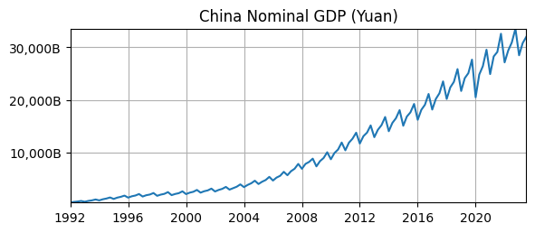

Is it stationary?

No, there is an exponential time trend, i.e., the mean is not constant.
No, the variance is smaller at the beginning that the end.

Seasonality¶

We know that we can remove seasonality with a difference with lag 4.
But we could also explicitly model seasonality as its own ARMA process.
Let’s use the PACF to determine what the AR order of the seasonal component might be.
First, let’s take $\log$ to remove the exponential trend.

# Scientific computing
import numpy as np
# Remove exponential trend
df['loggdp'] = np.log(df['gdp'])

# Partial auto-correlation function
from statsmodels.graphics.tsaplots import plot_pacf as pacf
# Plot Autocorrelation Function
fig, ax = plt.subplots(figsize=(6.5,2))
pacf(df['loggdp'],ax); ax.grid(); ax.autoscale(tight=True)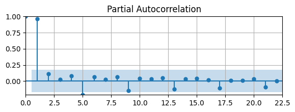

PACF is significant at lags 1 and 5 (and also almost at lags 9, 13,...)
i.e., this shows the high autocorrelation at a quarterly frequency
You could model the seasonality as $y_{s,t} = \phi_{s,0} + \phi_{s,4} y_{s,t-4} + \varepsilon_{s,t}$ (more on this later)

First Difference¶

# Year-over-year growth rate
df['d1loggdp'] = 100*(df['loggdp'] - df['loggdp'].shift(4))

# Plot
fig, ax = plt.subplots(figsize=(6.5,2));
ax.plot(df['d1loggdp']);
ax.set_title('China Nominal GDP Growth Rate (Year-over-year)');
ax.yaxis.set_major_formatter('{x:.0f}%')
ax.grid(); ax.autoscale(tight=True)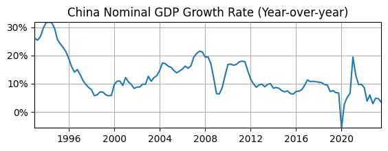

Does it look stationary?

Maybe not, it might have a downward time trend.
Maybe not, the volatility appears to change over time.
Maybe not, the autocorrelation looks higher at the beginning than end of sample.

# Auto-correlation function
from statsmodels.graphics.tsaplots import plot_acf as acf
# Plot Autocorrelation Function
fig, ax = plt.subplots(figsize=(6.5,2))
acf(df['d1loggdp'].dropna(),ax)
ax.grid(); ax.autoscale(tight=True)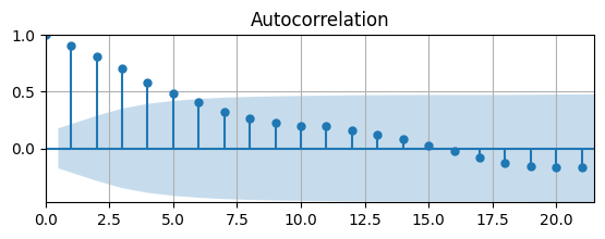

The ACF tapers quickly, but starts to become non-zero for long lags.
The AC is significantly different from zero for 4 lags. Let’s check the PACF to see if we can determine the order of an AR model.

# Plot Autocorrelation Function
fig, ax = plt.subplots(figsize=(6.5,1.5))
pacf(df['d1loggdp'].dropna(),ax)
ax.grid(); ax.autoscale(tight=True);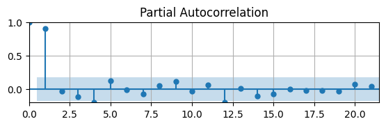

The PACF suggests to estimate an AR(1) model.
If we assume this first-differenced data is stationary and estimate an AR(1) model, what do we get?

# ARIMA model
from statsmodels.tsa.arima.model import ARIMA
# Define model
mod0 = ARIMA(df['d1loggdp'],order=(1,0,0))
# Estimate model
res = mod0.fit(); summary = res.summary()
# Print summary tables
tab0 = summary.tables[0].as_html(); tab1 = summary.tables[1].as_html(); tab2 = summary.tables[2].as_html()
#print(tab0); print(tab1); print(tab2)

Dep. Variable:	VALUE	No. Observations:	123
Model:	ARIMA(1, 0, 0)	Log Likelihood	-289.294

	coef	std err	z	P>\|z\|	[0.025	0.975]
const	12.9494	2.811	4.606	0.000	7.440	18.459
ar.L1	0.9399	0.026	36.315	0.000	0.889	0.991
sigma2	6.3511	0.348	18.243	0.000	5.669	7.033

Heteroskedasticity (H):	3.71	Skew:	0.11
Prob(H) (two-sided):	0.00	Kurtosis:	12.03

The residuals might be heteroskedastic, i.e., their volatility varies over time.
The kurtosis of the residuals indicate they are not normally distributed.
That suggests that data might still be non-stationary and need to be differenced again.

Second Difference¶

# Second difference
df['d2loggdp'] = df['d1loggdp'] - df['d1loggdp'].shift(1)
# Plot
fig, ax = plt.subplots(figsize=(6.5,1.5));
ax.plot(df['d2loggdp']); ax.set_title('Difference of China Nominal GDP Growth Rate')
ax.yaxis.set_major_formatter('{x:.0f}pp')
ax.grid(); ax.autoscale(tight=True)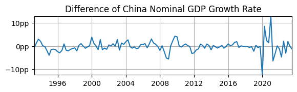

Does it look stationary?

Yes, the sample mean appears to be 0.
Yes, the volatility appears fairly constant over time, except during COVID.
Yes, the autocorrelation also appears fairly constant over time, at least until COVID.

# Plot Autocorrelation Function
fig, ax = plt.subplots(figsize=(6.5,2.5))
acf(df['d2loggdp'].dropna(),ax)
ax.grid(); ax.autoscale(tight=True)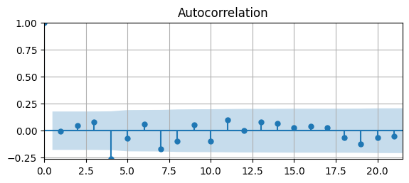

Estimation¶

# ARIMA model
from statsmodels.tsa.arima.model import ARIMA
# Define model
mod0 = ARIMA(df['loggdp'],order=(1,2,0))
mod1 = ARIMA(df['d1loggdp'],order=(1,1,0))
mod2 = ARIMA(df['d2loggdp'],order=(1,0,0))

# Estimate model
res = mod0.fit(); summary = res.summary()
# Print summary tables
tab0 = summary.tables[0].as_html(); tab1 = summary.tables[1].as_html(); tab2 = summary.tables[2].as_html()
#print(tab0); print(tab1); print(tab2)

Estimation Results ARIMA( $1,2,0$ )¶

Dep. Variable:	VALUE	No. Observations:	127
Model:	ARIMA(1, 2, 0)	Log Likelihood	49.700

	coef	std err	z	P>\|z\|	[0.025	0.975]
ar.L1	-0.6646	0.076	-8.722	0.000	-0.814	-0.515
sigma2	0.0263	0.004	6.541	0.000	0.018	0.034

Heteroskedasticity (H):	0.64	Skew:	-0.84
Prob(H) (two-sided):	0.15	Kurtosis:	2.35

Warning: the AR coefficient estimate is negative!
i.e., the way this time series has been differenced, the resulting series would flip from positive to negative every period.
Why? ARIMA has taken the first difference at 1 lag, instead of lag 4, so the seasonality has not been removed.

Estimation Results ARIMA( $1,1,0$ )¶

Dep. Variable:	VALUE	No. Observations:	123
Model:	ARIMA(1, 1, 0)	Log Likelihood	-287.368

	coef	std err	z	P>\|z\|	[0.025	0.975]
ar.L1	0.0024	0.045	0.053	0.958	-0.087	0.091
sigma2	6.5086	0.361	18.042	0.000	5.802	7.216

Heteroskedasticity (H):	4.22	Skew:	0.32
Prob(H) (two-sided):	0.00	Kurtosis:	12.12

AR coefficient estimate is not statistically significantly different from 0.
That is consistent with the ACF plot, so AR(1) is model is not the best choice.

Estimation Results ARIMA( $1, 0, 0$ )¶

Dep. Variable:	VALUE	No. Observations:	122
Model:	ARIMA(1, 0, 0)	Log Likelihood	-287.042

	coef	std err	z	P>\|z\|	[0.025	0.975]
const	-0.1863	0.231	-0.806	0.420	-0.639	0.267
ar.L1	-0.0025	0.045	-0.055	0.956	-0.092	0.087
sigma2	6.4739	0.357	18.126	0.000	5.774	7.174

Heteroskedasticity (H):	4.34	Skew:	0.32
Prob(H) (two-sided):	0.00	Kurtosis:	12.10

These results are nearly identical to estimating the ARIMA( $1,1,0$ ) with first-differenced data.
i.e., once you remove seasonality, you can difference your data manually or have ARIMA do it for you.

ARIMA `seasonal_order`¶

statsmodels ARIMA also has an argument to specify a model for seasonality.
Above, a first difference at lag 4 removed the seasonality.
seasonal_order=(P,D,Q,s) is the order of seasonal model for the AR parameters, differences, MA parameters, and periodicity ( $s$ ) .
We saw the periodicity of the seasonality in the data was 4 (and confirmed that with the PACF).
Let’s model the seasonality as an ARIMA( $1,1,0$ ) (since the seasonal component is strongly autocorrelated and the data is integrated) with periodicity of 4.
Then we can we estimate an ARIMA( $1,1,0$ ) using just $\log(GDP)$

mod3 = ARIMA(df['loggdp'],order=(1,1,0),seasonal_order=(1,1,0,4))
# Estimate model
res = mod3.fit(); summary = res.summary()
# Print summary tables
tab0 = summary.tables[0].as_html(); tab1 = summary.tables[1].as_html(); tab2 = summary.tables[2].as_html()
#tab0 = summary.tables[0].as_text(); tab1 = summary.tables[1].as_text(); tab2 = summary.tables[2].as_text()
#print(tab0); print(tab1); print(tab2)

Dep. Variable:	VALUE	No. Observations:	127
Model:	ARIMA(1, 1, 0)x(1, 1, 0, 4)	Log Likelihood	278.588

	coef	std err	z	P>\|z\|	[0.025	0.975]
ar.L1	0.0024	0.048	0.050	0.960	-0.092	0.096
ar.S.L4	-0.2598	0.043	-6.034	0.000	-0.344	-0.175
sigma2	0.0006	3.64e-05	16.652	0.000	0.001	0.001

Heteroskedasticity (H):	3.09	Skew:	-0.49
Prob(H) (two-sided):	0.00	Kurtosis:	10.65

The estimates for the AR parameter is the same as estimating an ARIMA(1,1,0) with first-differenced $\log(GDP)$ at lag 4.
There is an additional AR parameter for the seasonal component ar.S.L4, i.e., we’ve controlled for the seasonality.
While you can do this, it’s more transparent to remove seasonality by first differencing, then estimate an ARIMA model.

Summary¶

ARMA Model¶

Key Aspects¶

Integration¶

I(2)I(2)I(2) Example¶

Seasonality¶

First Difference¶

Second Difference¶

Estimation¶

Estimation Results ARIMA(1,2,01,2,01,2,0)¶

Estimation Results ARIMA(1,1,01,1,01,1,0)¶

Estimation Results ARIMA(1,0,01, 0, 01,0,0)¶

ARIMA seasonal_order¶

$I(2)$ Example¶

Estimation Results ARIMA( $1,2,0$ )¶

Estimation Results ARIMA( $1,1,0$ )¶

Estimation Results ARIMA( $1, 0, 0$ )¶

ARIMA `seasonal_order`¶