Jupyter Notebook

by Professor Throckmorton
for Intermediate Macro
W&M ECON 304
Slides

This cell contains Markdown with the title (i.e., a section title preceded by #) and other important information.

Summary¶

This Jupyter Notebook contains cells with examples of Markdown, $\LaTeX$ , and Python. These are versatile tools and the output is easy to create, read, and share.

Jupyter Hub¶

Follow these steps to open this notebook on Jupyter Hub so you can see how it works and modify it.

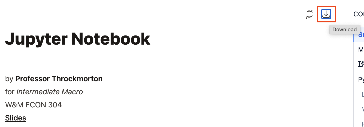
Download this notebook by clicking on the download button in the upper right and selecting “jupyter-notebook.ipynb”.
Log in to https://jupyterhub.wm.edu using you W&M credentials. (Select the default server, if prompted).

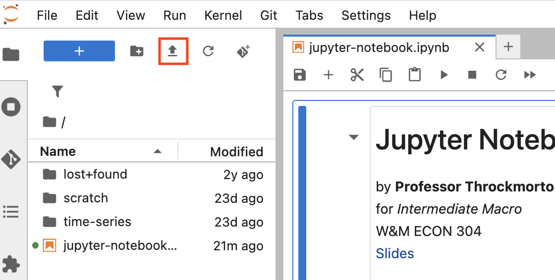
Upload the notebook to your server and double click/tap on the notebook to open it in a tab.

Markdown¶

Markdown is a simple and easy-to-use markup language you can use to format virtually any document. For Markdown basic syntax, please see https://www.markdownguide.org/basic-syntax/.

You can choose whether a cell contains Markdown or Code using the dropdown menu in the toolbar.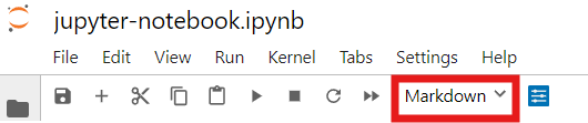

Note: I embeded this screenshot by simply copying and pasting the image into this Markdown cell. You may also save images in a/the sub/directory where the notebook is located and embed them, e.g., ![toolbar screenshot](jupyter-notebook-toolbar.png).

$\LaTeX$ ¶

You can typeset $\LaTeX$ in a Markdown cell (and also when labeling plots in Python). Here is a $\LaTeX$ math cheat sheet.

$\LaTeX$ surrounded by a single dollar sign, $...$ , is typeset inline, e.g., $y = x^2$ becomes $y = x^2$ . However, $\LaTeX$ surrounded by double dollar signs, $$...$$, is typeset on a separate line. For example, the Gaussian function, or the normal distribution’s probability density function (PDF), is

f(x) = \frac{1}{\sqrt{2\pi\sigma^2}}\exp\left\{\frac{-(x-\mu)^2}{2\sigma^2}\right\}.

(1)

is the result of

$$
  f(x) = \frac{1}{\sqrt{2\pi\sigma^2}}\exp\left\{\frac{-(x-\mu)^2}{2\sigma^2}\right\}.
$$

If you want to list a system of $N$ equations, then I recommend this syntax:

\begin{gather*}
    u(c,\ell) = \log(c) + \chi \log(\ell), \\
    \ell = 1 - n, \\
    c + i + g = f(k,n), \\
    f(k,n) = k^\alpha n^{1-\alpha}.
\end{gather*}

which looks like

\begin{gather*} u(c,\ell) = \log(c) + \chi \log(\ell), \\ \ell = 1 - n, \\ c + i + g = f(k,n), \\ f(k,n) = k^\alpha n^{1-\alpha}. \end{gather*}

(2)

Python¶

Libraries¶

The following code cell contains Python that imports libraries for plotting (matpotlib) and scientific computing (numpy). Then it sets a random number generator seed and assigns it to rng. A Python program will always begin with a header like this.

# Import libraries
#   Plotting
import matplotlib.pyplot as plt
#   Scientific computing
import numpy as np

# Set rng seed
rng = np.random.default_rng(seed=0)

Variables¶

The following code cell assigns the sample size to T and randomly generated data from a standard normal distribution to eps, i.e., $\varepsilon_t \overset{i.i.d.}{\sim} N(0,1)$ ( $\varepsilon_t$ is a random variable with a standard normal distribution that is independently and identically distributed across time). eps is also known as white noise data.

# Sample size
T = 201
# White noise data
eps = rng.standard_normal(T)

Histogram¶

The following cell will create a histogram of eps. If we weren’t thinking about eps as a time series variable, then the histogram could represent the distribution of the variable in the cross section dimension.

#   Plot histogram
plt.figure(figsize=(6.5,3))
plt.hist(eps,edgecolor='black',density='true')
plt.xlabel('White-noise data')
plt.ylabel('probability')
plt.grid()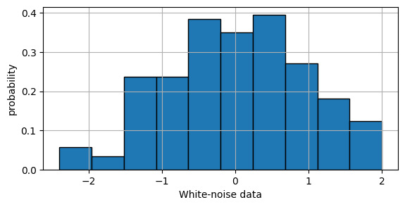

Time series¶

But since we want to think of eps as a time series variable, we should plot it as a function of time.

#   Plot time series
plt.figure(figsize=(6.5,3))
plt.plot(eps)
plt.title('White-noise data')
plt.xlabel('Time')
plt.xlim([0,T-1])
plt.grid()

Slides¶

Slides are easily created from a Jupyter Notebook (via nbconvert and reveal.js). For example, see Jupyter Notebook Slides.

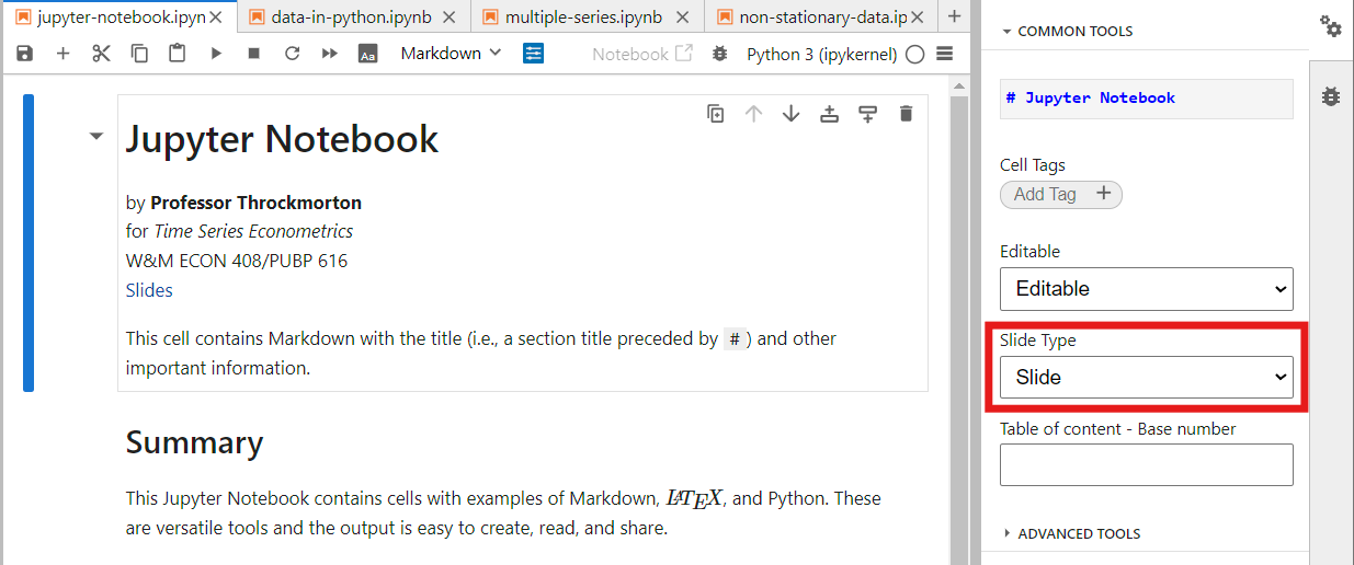
Open the property inspector by clicking the double gears in the upper-right-hand corner, and assign the “Slide Type” field.

“Slide” starts a new slide
“Fragment” does not create a new slide and instead hides the content until the presenter increments forward

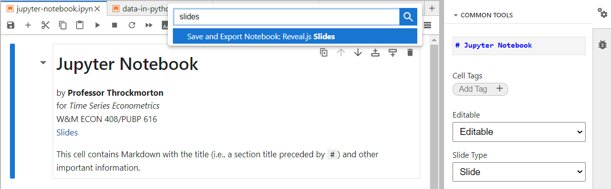
Press ctrl/command+shift+c (to open the command palette) and type “slides”. Press enter or click “Save and Export Notebook: Reveal.js Slides”. Alternatively, you can run the following from a terminal, or command line interface (CLI),
```
jupyter nbconvert 'jupyter-notebook.ipynb' --to slides --embed-images
```
Save the html file, which you can then open in any browser.

Conclusion¶

Jupyter Notebooks are versatile tools to display, run, and view the output of programs in Python (or other languages), to typeset math expressions in $\LaTeX$ , and to format text and analysis in Markdown.
Furthermore, Jupyter Notebooks are easily converted to presentation slides with the built-in support for reveal.js.

Notebooks

Jupyter and Python