Unit Roots
by Professor Throckmorton
for Time Series Econometrics
W&M ECON 408
Slides
Summary
The presence of unit roots make time series non-stationary.
Trend Stationarity: A trend-stationary time series has a deterministic time trend and is stationary after the trend is removed.
Difference Stationarity: A difference-stationary time series has a stochastic time trend and becomes stationary after differencing.
Unit root tests, e.g., the augmented Dickey-Fuller test (ADF test) are used to detect the presence of a unit root in a time series.
Unit root tests help determine if differencing is required to achieve stationarity, suggesting a stochastic time trend.
If an AR model has a unit root, it is called a unit root process, e.g., the random walk model.
AR() Polynomial
Consider the AR() model:
Whether an AR() produces stationary time series depends on the parameters , e.g., for AR(1),
This can be written in terms of an AR polynomial with the lag operator, , defined as
Define the AR polynomial as
Unit Roots of AR()
To find the roots of an AR(), set and solve for (which is sometimes complex), and the number of roots will equal the order of the polynomial.
An AR() has a unit root if the modulus of any of the roots equal 1.
For each unit root, the data must differenced to make it stationary, e.g., if there are 2 unit roots then the data must be differenced twice.
If the modulus of all the roots exceeds 1, then the AR() is stationary.
Examples
AR(1):
Thus, an AR(1) has a unit root, , if .
If , then is a random walk model that produces non-stationary time series.
But the first difference is stationary (since is white noise).
Note if , then and the AR(1) is stationary.
AR(2): or
The AR(2) polynomial has a factorization such that with roots and
Thus, an AR(2) model is stationary if and .
Given the mapping and , we can prove that the modulus of both roots exceed 1 if
Unit Root Test
The augmented Dickey-Fuller test (ADF test) has hypotheses
: The time series has a unit root, indicating it is non-stationary.
: The time series does not have a unit root, suggesting it is stationary.
Test Procedure
Write an AR() model with the AR polynomial, .
If the AR polynomial has a unit root, it can be written as where .
Define .
An AR() model with a unit root is then .
Thus, testing for a unit root is equivalent to the test vs. in
Intuition: A stationary process reverts to its mean, so should be negatively related to .
adfuller
In
statsmodels, the functionadfuller()conducts an ADF unit root test.If the p-value is smaller than 0.05, then the series is probably stationary.
# ADF Test
from statsmodels.tsa.stattools import adfuller
# Function to organize ADF test results
def adf_test(data):
    keys = ['Test Statistic','p-value','# of Lags','# of Obs']
    values = adfuller(data)
    test = pd.DataFrame.from_dict(dict(zip(keys,values[0:4])),
                                  orient='index',columns=[data.name])
    return test
ADF test results
test = adf_test(df['d1loggdp'].dropna())
#print(test.to_markdown())| d1loggdp | |
|---|---|
| Test Statistic | -3.1799 |
| p-value | 0.0211781 |
| # of Lags | 4 |
| # of Obs | 118 |
The p-value < 0.05, reject the null hypothesis that the process is non-stationary.
The number of lags is chosen by minimizing the Akaike Information Criterion (AIC) (more on that soon).
dl = []
for column in df.columns:
    test = adf_test(df[column].dropna())
    dl.append(test)
results = pd.concat(dl, axis=1)
#print(results.to_markdown())| gdp | loggdp | d1loggdp | d2loggdp | |
|---|---|---|---|---|
| Test Statistic | 4.294 | -1.27023 | -3.1799 | -6.54055 |
| p-value | 1 | 0.642682 | 0.0211781 | 9.37063e-09 |
| # of Lags | 7 | 8 | 4 | 3 |
| # of Obs | 119 | 118 | 118 | 118 |
China GDP has a unit root after taking
log.China GDP is probably stationary after removing seasonality and converting to growth rate (p-value < 0.05).
Second difference of China GDP is almost certainly stationary.
U.S. Unemployment Rate
# Read Data
fred_api_key = pd.read_csv('fred_api_key.txt', header=None)
fred = Fred(api_key=fred_api_key.iloc[0,0])
data = fred.get_series('UNRATE').to_frame(name='UR')
# Plot
fig, ax = plt.subplots(figsize=(6.5,2));
ax.plot(data.UR); ax.set_title('U.S. Unemployment Rate');
ax.yaxis.set_major_formatter('{x:,.1f}%')
ax.grid(); ax.autoscale(tight=True)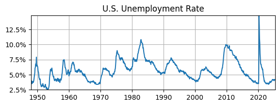
adf_UR = adf_test(data.UR)
print(adf_UR)
UR
Test Statistic -3.918852
p-value 0.001900
# of Lags 1.000000
# of Obs 928.000000
ADF test suggests that U.S. unemployment rate is stationary (p-value < 0.05).
This doesn’t necessarily contradict the ACF, which suggested the UR might be non-stationary, i.e., we couldn’t tell with certainty.
This result may not be surprising since modeling the UR as AR(1) led to an estimate of the AC parameter that was less than 1, i.e., it was not close to a random walk.
Order Determination
There are a lot of possible choices for the orders of an ARIMA() model.
Even if the data is not seasonal and already stationary, there are plenty of possibilities for an ARMA() model.
In the ADF tests above,
adfullerselected the lags for an AR() model for the first-differenced time series to test for a unit root.How do we select the best orders for an ARMA() model?
Information Criterion
Information criteria are used for order determination (i.e., model selection) of ARMA() models.
In
adfuller, the default method to select lags is the Akaike Information Criterion (AIC). Another choice is the Bayesian Information Criterion (BIC) (a.k.a. Schwarz Information Criterion (SIC)).The AIC and BIC are commonly used in economics research using time series data.
But there are other choices as well, e.g., the Hannan-Quinn Information Criterion (HQIC).
The goal of AIC, BIC, and HQIC is to estimate the out-of-sample mean square prediction error, so a smaller value indicates a better model.
AIC vs. BIC
Let be the maximized log-likelihood of the model, be the number of estimated parameters, and be the sample size of the data.
The key difference is that
AIC has a tendency to overestimate the model order.
BIC places a bigger penalty on model complexity, hence the best model is parsimonious relative to AIC.
Consistency, i.e., as the sample size increases does the information criteria select the true model?
AIC is not consistent, but it is asymptotically efficient, which is relevant for forecasting (more on that much later).
BIC is consistent.
When AIC and BIC suggest different choices, most people will choose the parsimonious model using the BIC.
Likelihood Function
Likelihood function: Probability of the observed time series data given a model and its parameterization.
Maximum Likelihood Estimation: For a given model, find the parameterization that maximizes the likelihood function, i.e., such that the observed time series has a higher probability than with any other parameterizaiton.
The likelihood function is the joint probability distribution of all observations.
In ARMA/ARIMA models, the likelihood function is just a product of Gaussian/normal distributions since that is the distribution of the errors/innovations.
Order determination/model selection:
Given some time series data and a menu of models, which model has the highest likelihood and is relatively parsimonious?
e.g., for each AR model we can compute the ordinary least squares estimates and then the value of the likelihood function for that parameterization.
Example
Assume an MA(2) model: , where are i.i.d. normal errors. Note: by construction is uncorrelated with
The likelihood function is the joint probability distribution of the observations , given parameters of the model
where is the conditional normal density
Combining the previous expressions and substituting out for yields
The log-likelihood function (i.e., taking natural log converts a product to a sum) is
To estimate , maximize this log-likelihood function, i.e., .
Because is nonlinear in the parameters, numerical methods such as nonlinear optimization or the conditional likelihood approach are used in practice.