RBC Model
by Professor Throckmorton
for Time Series Econometrics
W&M ECON 408
Slides
Summary
Introduce a nonlinear theoretical model of business cycles.
Get the equilibrium conditions and linear the system of equations.
Solve the linear system, i.e., express (observable) endogenous variables as functions of (hidden) state variables.
Estimate the state vector with the Kalman filter.
The following example is a simplified exposition of Chad Fulton’s RBC example in Python here: https://
www .chadfulton .com /topics /estimating _rbc .html
The Model
A social planner chooses how much to consume, work, and invest, , to maximize present value lifetime utility
subject to:
resource constraint:
capital accumulation:
production function:
Total factor productivity (TFP):
where
is an expectation operator conditional data through time , i.e., it’s a forecast because TFP is random/stochastic
Parameters
This model has the following parameters
| Parameter | Description | Parameter | Description |
|---|---|---|---|
| Discount factor | TFP shock persistence | ||
| Marginal disutility of work | TFP shock variance | ||
| Capital depreciation rate | Capital-share of output |
Example parameterization
| Parameter | Value | Parameter | Value |
|---|---|---|---|
| 0.95 | 0.85 | ||
| 3 | 0.04 | ||
| 0.025 | 0.36 |
The ultimate goal is to estimate (some of) these parameters.
Equilibrium
The RBC model is a constrained optimization problem which can be written as a Lagrangian with the following first order conditions (i.e., equilibrium conditions).
In equilibrium, the marginal benefit (i.e., utility) of a unit of consumption today equals the marginal cost (i.e., lost future utility) forgoing the future return on a unit of investment:
where is the marginal utility of consumption and is the marginal product of capital.
In equilibrium, the marginal benefit (i.e., utility) of work equals the marginal cost (i.e., disutility) of work.
where is the marginal product of work.
Including the constraints completes the nonlinear equilibrium system.
Linear System
The linearized equilibrium system of equations is
The state variables for this system are , i.e., the social planner needs to know those to make decisions at .
There are 8 variables, , which (importantly!) equals the number of equations.
This is a linear model with (rational) expectations/forecasts, i.e., the social planner forecasts with full understanding of the structure of the model, the initial conditions/state, , and the distribution of TFP.
A solution to the model expresses the endogenous variables as functions of the state variables .
We can obtain the solution with methods in Blanchard-Kahn (1980) or Chris Sims’ gensys.
The solution to the linear system is represented in state-space form.
Solution
Observation equation(s):
State equation(s):
Given the above parameterization, the solution is
| Parameter | Value |
|---|---|
| 0.534 | |
| 0.487 | |
| 0.884 | |
| 0.319 | |
| 0.36 |
Business Cycle Data
In the RBC model, where is the (constant) long-run equilibrium.
Q: What is the equivalent object in time series data with stochastic or time trends?
The Hodrick-Prescott (HP) filter is one (of many) mathematical tool(s) used to decompose a time series into:
: A smooth trend component capturing both time and stochastic trends
: A cyclical component, i.e., the object of interest for business cycle economists
In other words, we can express the data as percent changes from a “long run equilibrium”, , i.e., percent deviations from trend.
In business cycle research, other popular choices are the band-pass filter and Hamilton filter.
James Hamilton wrote a critque of the HP filter, and then created “a better alternative,” which now has over 2300 citations as of Spring 2026.
The HP filter finds the trend by solving a minimization problem:
First term: makes the trend close to the actual data.
Second term: penalizes sharp changes in the slope of the trend, enforcing smoothness.
influences the smoothness of the resulting trend
Small → Trend follows the data closely (e.g., wiggly trend with “sharp” changes).
Large → Trend is very smooth (e.g., nearly a straight line).
Common Choices for
for quarterly data
for monthly data
for annual data
Reading Data
# Libraries
from fredapi import Fred
import pandas as pd
# Setup acccess to FRED
fred_api_key = pd.read_csv('fred_api_key.txt', header=None).iloc[0,0]
fred = Fred(api_key=fred_api_key)
# Series to get
series = ['GDP','PRS85006023','PCE','GDPDEF','USREC']
rename = ['gdp','hours','cons','price','rec']
# Get and append data to list
dl = []
for idx, string in enumerate(series):
    var = fred.get_series(string).to_frame(name=rename[idx])
    dl.append(var)
    print(var.head(2)); print(var.tail(2))
gdp
1946-01-01 NaN
1946-04-01 NaN
gdp
2025-07-01 31098.027
2025-10-01 31422.526
hours
1947-01-01 117.931
1947-04-01 117.425
hours
2025-07-01 98.086
2025-10-01 97.910
cons
1959-01-01 306.1
1959-02-01 309.6
cons
2026-01-01 21511.8
2026-02-01 21615.1
price
1947-01-01 11.141
1947-04-01 11.299
price
2025-07-01 129.430
2025-10-01 130.624
rec
1854-12-01 1.0
1855-01-01 0.0
rec
2026-02-01 0.0
2026-03-01 0.0
# Concatenate data to create data frame (time-series table)
rawm = pd.concat(dl, axis=1, sort=False).sort_index()
# Resample/reindex to quarterly frequency
raw = rawm.resample('QE').last().dropna()
# real GDP
raw['rgdp'] = raw['gdp']/raw['price']
# real Consumption
raw['rcons'] = raw['cons']/raw['price']
# Display dataframe
display(raw)HP Filter
The vector of observable endogenous variables is , where and is the smooth trend from the HP filter.
# Hodrick-Prescott filter
from statsmodels.tsa.filters.hp_filter import hpfilter
# Smoothing parameter for quarterly data
lam = 1600
# Raw data to detrend
vars = ['rgdp','hours','rcons']
nvar = len(vars)
# Detrend raw data
data = pd.DataFrame()
for var in vars:
    cycle, trend = hpfilter(raw[var],lam)
    data[var] = 100*(raw[var]/trend - 1)
ax = data.plot(); ax.grid(); ax.set_title('Observables (% Dev. from Trend)')
ax.legend([r'Real GDP ($\hat y_t$)',r'Hours ($\hat n_t$)',r'Real PCE ($\hat c_t$)'],ncol=3);
fig = ax.get_figure(); fig.set_size_inches(6.5,2.5)
# Shade NBER recessions
usrec = rawm['3/31/1959':'12/31/2025']['rec']
ax.fill_between(usrec.index, -8.5, 5, where=usrec.values, color='k', alpha=0.2)
ax.autoscale(tight=True)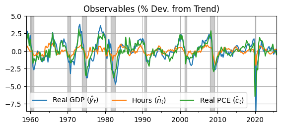
RBC Model in Python
Set the parameters in the state space model, which represents the solution to the linearized RBC model.
# Define the state space model
#  Parameters
phick = 0.534; phicz = 0.487
Tkk = 0.884; Tkz = 0.319
alpha = 0.36; rho = 0.85; sigma2 = 0.4;
Simplified Observation (Measurement) Equation: where
# Scientific computing
import numpy as np
# Observation equation
Z11 = 1 - (1-alpha)*phick/alpha
Z12 = 1/alpha - (1-alpha)*phicz/alpha
Z21 = 1 - phick/alpha
Z22 = (1-phicz)/alpha
Z31 = phick
Z32 = phicz
Z = np.array([[Z11,Z12],[Z21,Z22],[Z31,Z32]])
H = 1e-8*np.eye(nvar)
display(Z)
display(H)
array([[ 0.05066667, 1.912 ],
[-0.48333333, 1.425 ],
[ 0.534 , 0.487 ]])array([[1.e-08, 0.e+00, 0.e+00],
[0.e+00, 1.e-08, 0.e+00],
[0.e+00, 0.e+00, 1.e-08]])Simplified State (Transition) Equation: where
# Transition equation
F = [[Tkk,Tkz],[0,rho]]
Q = [[0,0],[0,sigma2]]
display(F)
display(Q)
[[0.884, 0.319], [0, 0.85]][[0, 0], [0, 0.4]]Kalman Filter
from statsmodels.tsa.statespace.kalman_filter import KalmanFilter
# Initialize the Kalman filter
kf = KalmanFilter(k_endog=nvar, k_states=2)
kf.design = Z
kf.obs_cov = H
kf.transition = F
kf.state_cov = Q
kf.selection = np.identity(2)
#   Initial state vector mean and covariance
kf.initialize_known(constant=np.zeros(2), stationary_cov=Q)
# Extract data from Dataframe as NumPy array
observations = np.array(data)
# Convert data to match the required type
observations = np.asarray(observations, order="C", dtype=np.float64)
# Bind the data to the KalmanFilter object
kf.bind(observations)
# Extract filtered state estimates
res = kf.filter()
filtered_state_means = res.filtered_state
filtered_state_covariances = res.filtered_state_cov
display(filtered_state_means.shape)
display(filtered_state_covariances.shape)(2, 268)(2, 2, 268)Filtered (Estimated) States
xhat = pd.DataFrame(filtered_state_means.T,index=data.index)
ax = xhat.plot(); ax.grid(); ax.set_title('Filtered States (% Dev. from Trend)')
fig = ax.get_figure(); fig.set_size_inches(6.5,2.5)
ax.legend([r'Capital ($\hat k_t$)',r'TFP ($\hat z_t$)'],ncol=2);
# Shade NBER recessions
ax.fill_between(usrec.index, -4, 2, where=usrec.values, color='k', alpha=0.2)
ax.autoscale(tight=True)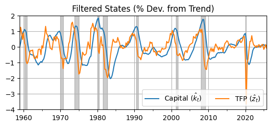
Source
import matplotlib.pyplot as plt
fig, axs = plt.subplots(2,figsize=(6.5,6)); fig.set_size_inches(8.5,6)
axs[0].plot(data); axs[0].grid(); axs[0].set_title('Observables (% Dev. from Trend)')
axs[0].legend([r'Real GDP ($\hat y_t$)',r'Hours ($\hat n_t$)',r'Real PCE ($\hat c_t$)'],ncol=3);
axs[0].fill_between(usrec.index, -8.5, 5, where=usrec.values, color='k', alpha=0.2)
axs[1].plot(xhat); axs[1].grid(); axs[1].set_title('States (% Dev. from Trend)')
axs[1].legend([r'Capital ($\hat k_t$)',r'TFP ($\hat z_t$)'],ncol=2);
axs[1].fill_between(usrec.index, -2, 2, where=usrec.values, color='k', alpha=0.2)
axs[0].label_outer(); axs[0].autoscale(tight=True); axs[1].autoscale(tight=True)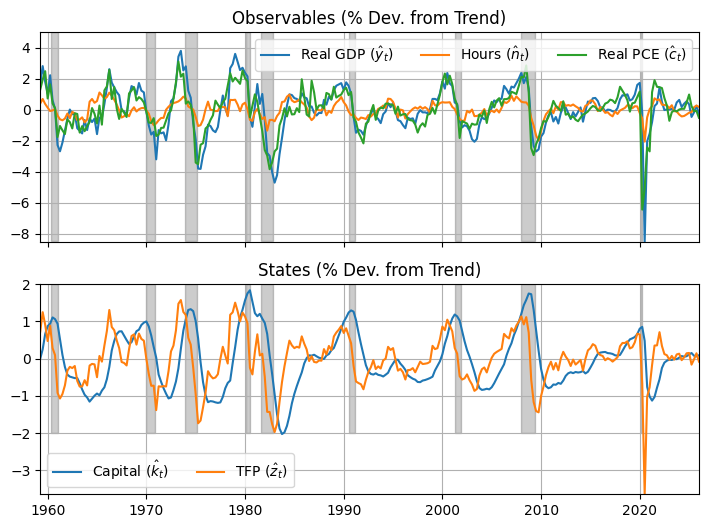
Parameter Estimation
loglike = res.llf
print(f"Log-likelihood: {loglike}")
Log-likelihood: -20803243748.869995
Kalman filter produces log likelihood for this parameterization
We could do a better job calibrating some parameters like the discount factor () and the labor preference parameter ()
Then we could search the parameter space for TFP process parameters, , that maximize the log likelihood.
This model is very simple.
We could change the utility function to add a risk aversion parameter.
We could add investment adjustment costs and variable capital utilization.
We could add demand shocks from preference shocks, government spending, or monetary policy.